Realtime visualization of 3D vector fields using CUDA
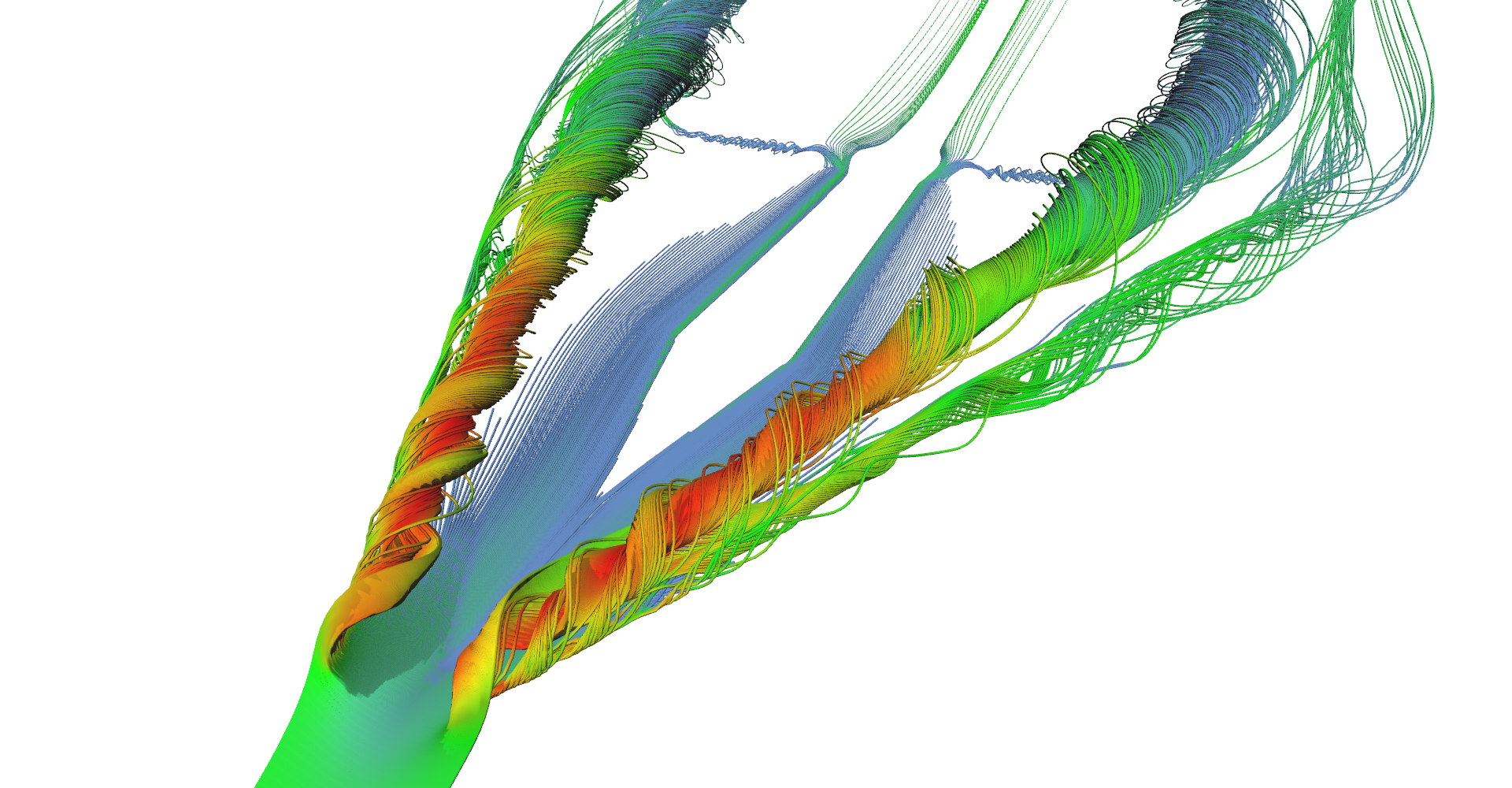
This project demonstrates visualization techniques like glyphs, stream lines, stream tubes, and stream surfaces, all done in real time. The key is an RK4 integrator implemented using CUDA that uses very fast texture lookup functions to access a vector field. This article contains more than 100 images and figures, commented code snippets, and source code available for download.
Source code is available on GitHub: NightElfik/Vector-field-visualization-using-cuda
1. Introduction#
Stream tubes seeded near the tip of the delta-wing. 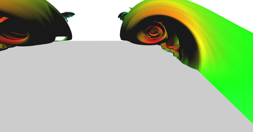
Detail on the stream surface of the primary vortex. 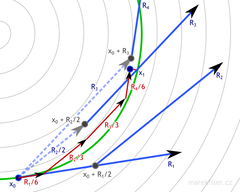
Explanation of Runge–Kutta 4 integration. 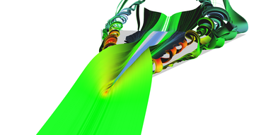
Stream surface combined with stream lines. 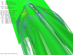
Benchmark of the system. 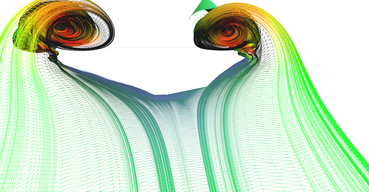
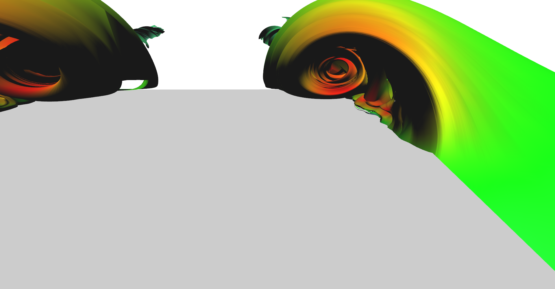
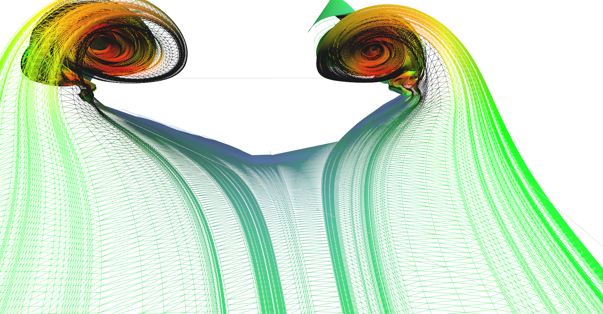
Adaptive triangulation.
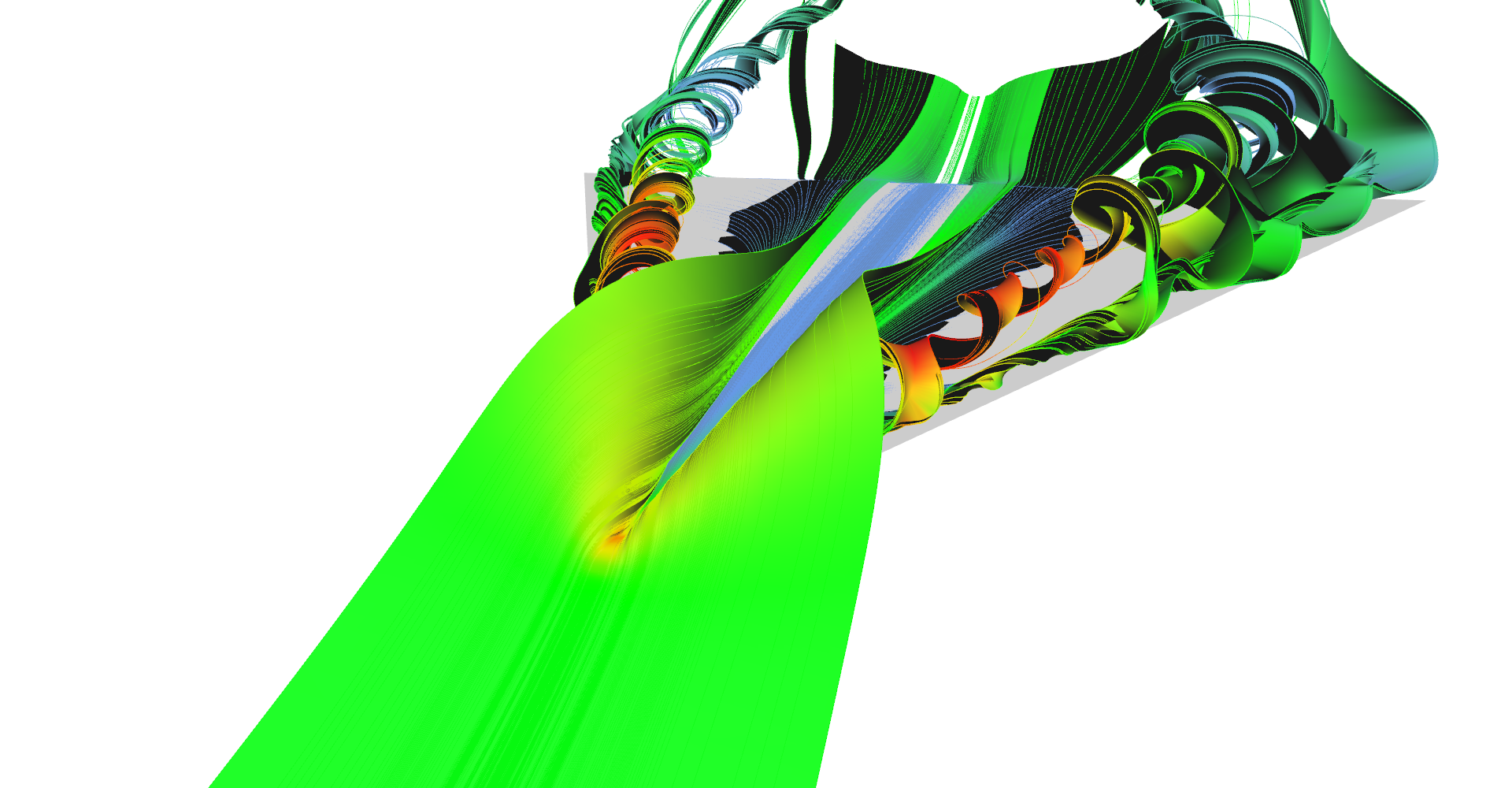
Vector field visualization is a special case of flow visualization where the flow is "frozen" (in time). Such a "frozen" fluid flow can be represented as a vector field which gives us information about the speed and direction of the fluid at any given point. For practical reasons we usually have only a finite number of samples within the observed volume and a vector at an arbitrary location is computed using some kind of interpolation. Flow visualizations are important in all kinds of engineering like airplane or car design.
The topic of this project is visualization of vector field using various techniques like stream lines, stream tubes, stream surfaces and glyphs. This project was the final assignment in Introduction to Scientific Visualization class (CS 530). The assignment was meant to be implemented using an open-source library called Visualization Toolkit (VTK) but I decided to implement it completely from scratch hoping that I will learn a lot of new things which turned out to be very true. Also, my implementation uses CUDA for acceleration of computation on GPU to achieve interactivity. Full source code is available on GitHub.
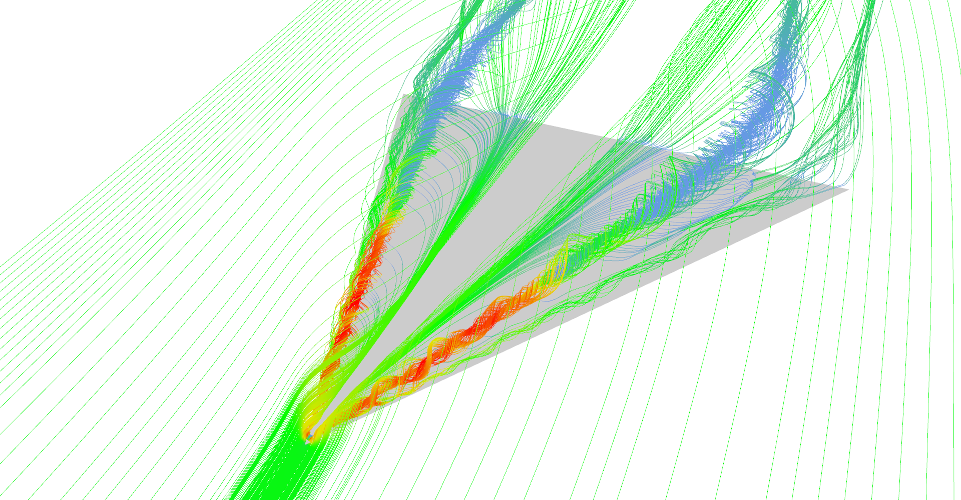 Figure 1: Stream line visualization of air flow around delta wing.
Dataset#
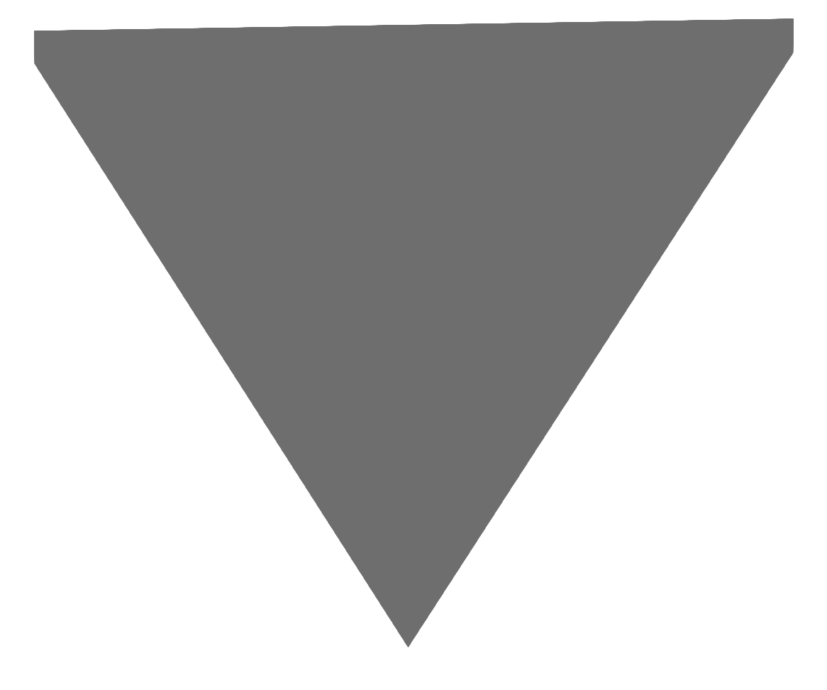
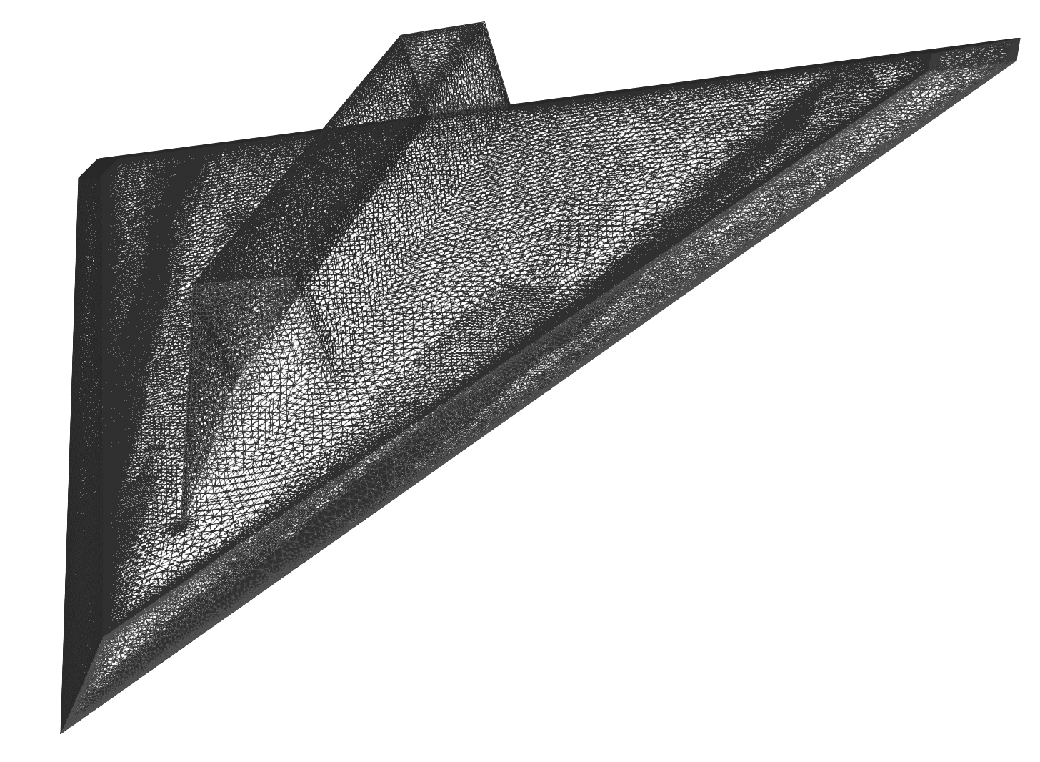
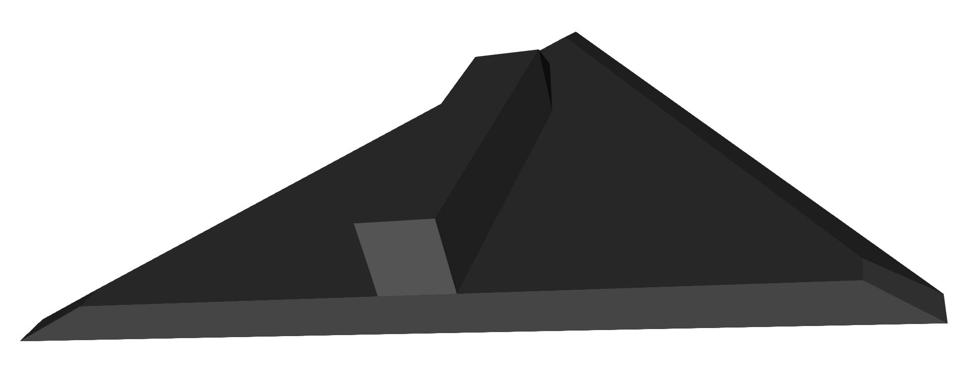
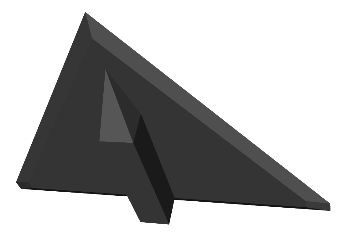
The input for this visualization is a pre-computed 3D vector field of air flowing around delta-wing (see Fig. Figure 2). I believe that dataset which was given to us is available somewhere on the Internet however I had no luck in finding it.
I was working with two versions of the dataset:
- Small 400×200×150 (138 MB raw)
- Large 800×400×300 (1.1 GB raw)
The only catch of the dataset is that spacing of samples is 1×1×0.5 which makes absolute size of the last dimension two times smaller.
All images on this page were made using the large dataset.
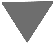
Delta-wing model from the top. 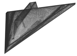
Delta-wing wireframe model - mesh is pretty detailed. 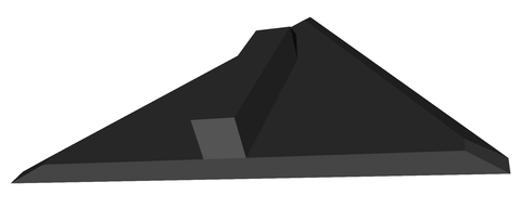
Delta-wing model from the bottom - you can see the aerodynamic box on the bottom. 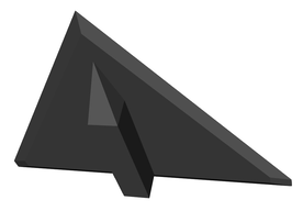
Another picture of delta-wing model from the bottom.
Loading input#
Input dataset is in NRRD file format which is basically plain text header information followed by raw uncompressed data.
In my case the data is a 3D array of 3D floating-point vectors which makes it a 4D array of floats.
This 4D array is linearized with the first dimension varying the fastest.
The header from the large dataset is shown in Code listing 1.
The complete NRRD file format specification can be found at http://teem.sourceforge.net/nrrd/format.html.
1
2
3
4
5
6
7
8
9
NRRD0001
type: float
dimension: 4
sizes: 3 800 400 300
spacings: 1 1.0012515783 1.0025062561 0.50167226791
axis mins: 0 -150 -200 -50
labels: "Vx;Vy;Vz" "x" "y" "z"
endian: little
encoding: raw
Because I decided to not use VTK, I had to write my own reader but it was pretty straightforward. The only thing I would like to mention here is how easily binary data can be read from a binary stream. Code listing 2 shows a main cycle of reading vector field.
Notice that I am using 4D vector (instead of 3D) for storing the vector field. The fourth dimension is used for storing vector magnitude, details are explained in the next section.
The only catch here is endianness. I am silently assuming that endianness of the file matches endianness of my CPU which is true, both are little-endian.
1
2
3
4
5
6
7
8
9
10
11
12
13
std::ifstream inputStream(filePath, std::ios::binary);
// Reading of header information skipped.
// ... float3 size initialized with size of VF
size_t totalSize = size.x * size.y * size.z;
float4* data = new float4[totalSize];

for (size_t i = 0; i < totalSize; ++i) {
	float4* f4Ptr = &(data[i]);
	// Read x, y, z.
	inputStream.read((char*)f4Ptr, sizeof(float3));
	// Compute magnitude as w.
	curr->w = std::sqrtf(f4Ptr->x * f4Ptr->x + f4Ptr->y * f4Ptr->y + f4Ptr->z * f4Ptr->z);
}
Fast reading of volumetric data using CUDA#
The core of any visualization technique is reading values at any point within a given 3D vector field. Since the input is a discrete grid, linear interpolation is needed for reading a point which is not on the grid (basically 100% of the queries).
This is the first place where CUDA will kick in.
CUDA offers very fast functions for reading 3D textures with linear interpolation which is exactly what is needed here.
However the only supported types are float1, float2 or float4 (no float3) but this led to another advantage.
I've used fourth dimension of float4 for storing vector magnitudes which are computed while parsing data from file.
This will significantly speed up visualization.
The only disadvantage is that this will increase memory consumption by 1/3 which is quite a big deal when we are speaking about GPU memory.
Initialization of 3D texture and loading data to GPU is shown in Code listing 3. Reading of vector data at arbitrary position is as simple as:
1
float4 vector = tex3D(vectorFieldTex, x, y, z);
1
2
3
4
5
6
7
8
9
10
11
12
13
14
15
16
17
18
19
20
21
22
23
24
25
26
texture<float4, cudaTextureType3D, cudaReadModeElementType> vectorFieldTex;
cudaArray* d_volumeArray = nullptr;

void initCuda(const float4* h_volume, cudaExtent volumeSize) {
	// Allocate 3D array.
	cudaChannelFormatDesc channelDesc = cudaCreateChannelDesc<float4>();
	cudaMalloc3DArray(&d_volumeArray, &channelDesc, volumeSize);

	// Copy data to 3D array using pitched ptr.
	cudaMemcpy3DParms copyParams = {0};
	copyParams.srcPtr = make_cudaPitchedPtr((void*)h_volume,
		volumeSize.width * sizeof(float4), volumeSize.width, volumeSize.height);
	copyParams.dstArray = d_volumeArray;
	copyParams.extent = volumeSize;
	copyParams.kind = cudaMemcpyHostToDevice;

	// Set texture parameters.
	vectorFieldTex.normalized = false;
	vectorFieldTex.filterMode = cudaFilterModeLinear;
	vectorFieldTex.addressMode[0] = cudaAddressModeClamp;
	vectorFieldTex.addressMode[1] = cudaAddressModeClamp;
	vectorFieldTex.addressMode[2] = cudaAddressModeClamp;

	// Bind 3D array to 3D texture.
	cudaBindTextureToArray(vectorFieldTex, d_volumeArray, channelDesc);
}
Color gradient for magnitude visualization#
Magnitude of vectors is very important for visualization because it represents velocity of the air flow.
I chose a linear blue-green-red gradient to represent the magnitude where blue represents the lowest magnitude in the dataset and red the highest (Figure 3).
This gradient is stored and queried in the same fashion as main vector data.
Color values are saved in a 1D texture on GPU and CUDA command tex1D is used for fetching interpolated value.
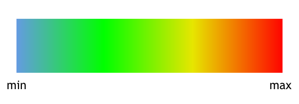 Figure 3: Color gradient used for visualization of vector magnitudes
OpenGL CUDA interoperability#
A great advantage of using CUDA in this type of application is that very little data needs to be transferred between CPU and GPU. The only data which needs to be transferred from CPU to GPU are start positions (seeds) and it is usually very few data (units of kilobytes). Results of CUDA computations are left in GPU memory and immediately displayed using VBOs.
Code listing 4 shows how shared VBOs are initialized. First, OpenGL VBO is created and then a CUDA buffer is obtained from the VBO. This ensures that both VBO pointer and CUDA device pointer will point to the same chunk of GPU memory.
Code listing 5 shows simplified usage of interoperability between OpenGL VBOs and CUDA.
Function allocate just allocates needed memory for CUDA kernel invocation (shown in Code listing 4).
Function recompute invokes CUDA kernel which will write results to provided memory which is VBO mapped buffer.
Function cudaGraphicsMapResources tells GPU that this memory will be accessed by CUDA and if you try to use it with OpenGL before unmapping,
bad things will happen to you (e.g. your program).
Function cudaGraphicsResourceGetMappedPointer will retrieve device pointer from mapped VBO.
The last function in Code listing 5 called displayCallback will bind VBOs and render them.
Super fast, super efficient, I love it!
1
2
3
4
5
6
7
8
9
cudaError_t createCudaSharedVbo(GLuint* vbo, GLenum target, uint size,
		cudaGraphicsResource** cudaResource) {

	glGenBuffers(1, vbo);
	glBindBuffer(target, *vbo);
	glBufferData(target, size, 0, GL_DYNAMIC_DRAW);
	glBindBuffer(target, 0);
	return cudaGraphicsGLRegisterBuffer(cudaResource, *vbo, cudaGraphicsMapFlagsNone);
}
1
2
3
4
5
6
7
8
9
10
11
12
13
14
15
16
17
18
19
20
21
22
23
24
25
26
27
28
29
30
31
32
33
34
35
36
void allocate() {
	createCudaSharedVbo(&m_verticesVbo, GL_ARRAY_BUFFER,
		verticesCount * sizeof(float3), &m_cudaVerticesVboResource);
	createCudaSharedVbo(&m_colorsVbo, GL_ARRAY_BUFFER,
		verticesCount * sizeof(float3), &m_cudaColorsVboResource);
}

void recompute() {
	size_t bytesCount;
	float3* d_glyphs;
	cudaGraphicsMapResources(1, &m_cudaVerticesVboResource);
	cudaGraphicsResourceGetMappedPointer((void**)&d_glyphs, &bytesCount,
		m_cudaVerticesVboResource);

	float3* d_colors;
	cudaGraphicsMapResources(1, &m_cudaColorsVboResource);
	cudaGraphicsResourceGetMappedPointer((void**)&d_colors, &bytesCount,
		m_cudaColorsVboResource);

	runCudaKernel(..., d_glyphs, d_colors, m_glyphsCount, ...);

	cudaGraphicsUnmapResources(1, &m_cudaColorsVboResource);
	cudaGraphicsUnmapResources(1, &m_cudaVerticesVboResource);
}

void displayCallback() {
	glBindBuffer(GL_ARRAY_BUFFER, m_verticesVbo);
	glEnableClientState(GL_VERTEX_ARRAY);
	glVertexPointer(3, GL_FLOAT, 0, NULL);

	glBindBuffer(GL_ARRAY_BUFFER, m_colorsVbo);
	glEnableClientState(GL_COLOR_ARRAY);
	glColorPointer(3, GL_FLOAT, 0, NULL);

	glDrawArrays(GL_LINES, 0, 2 * m_glyphsCount.x * m_glyphsCount.y);
}
2. Visualization using glyphs#
A glyph is some marker, such as an arrow or line, used to visualize vector field (in our case). Visualization using glyphs is the easiest type of visualization and I did two types, lines and arrows. Both techniques are described in the following subsections.
Line glyphs for VF visualization#
Lines visualization is very simple to implement. For every point in a given plane it computes a line with orientation matching the vector field in given point and length of line and color are given by vector magnitude (flow intensity).
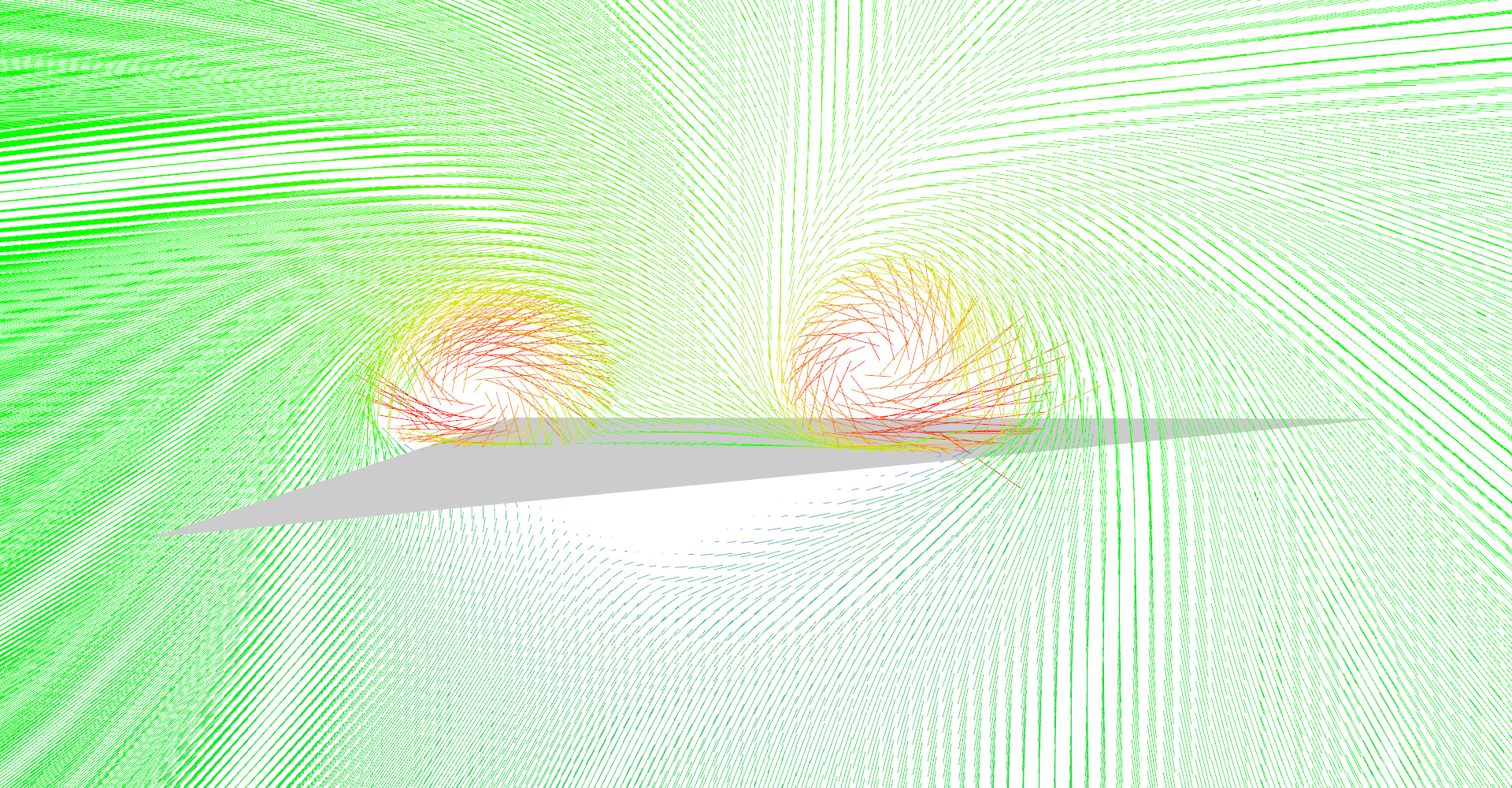
Code listing 6 shows a (simplified) kernel which computed lines in the YZ plane. X axis is the only degree of freedom of this visualization and can be controlled by the user. It might seem like a limitation but it is enough for dataset of delta-wing where air flow follows x-axis.
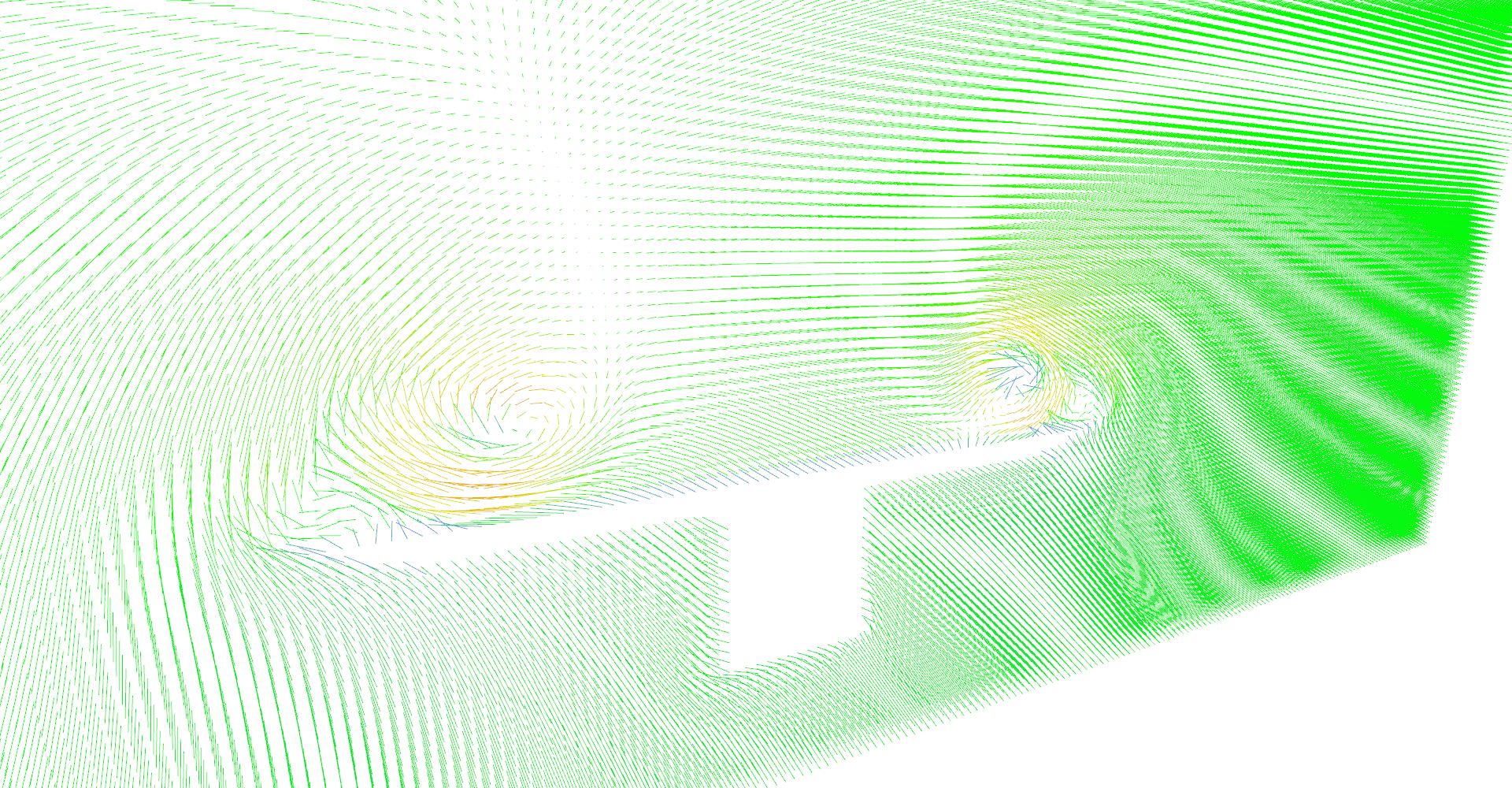
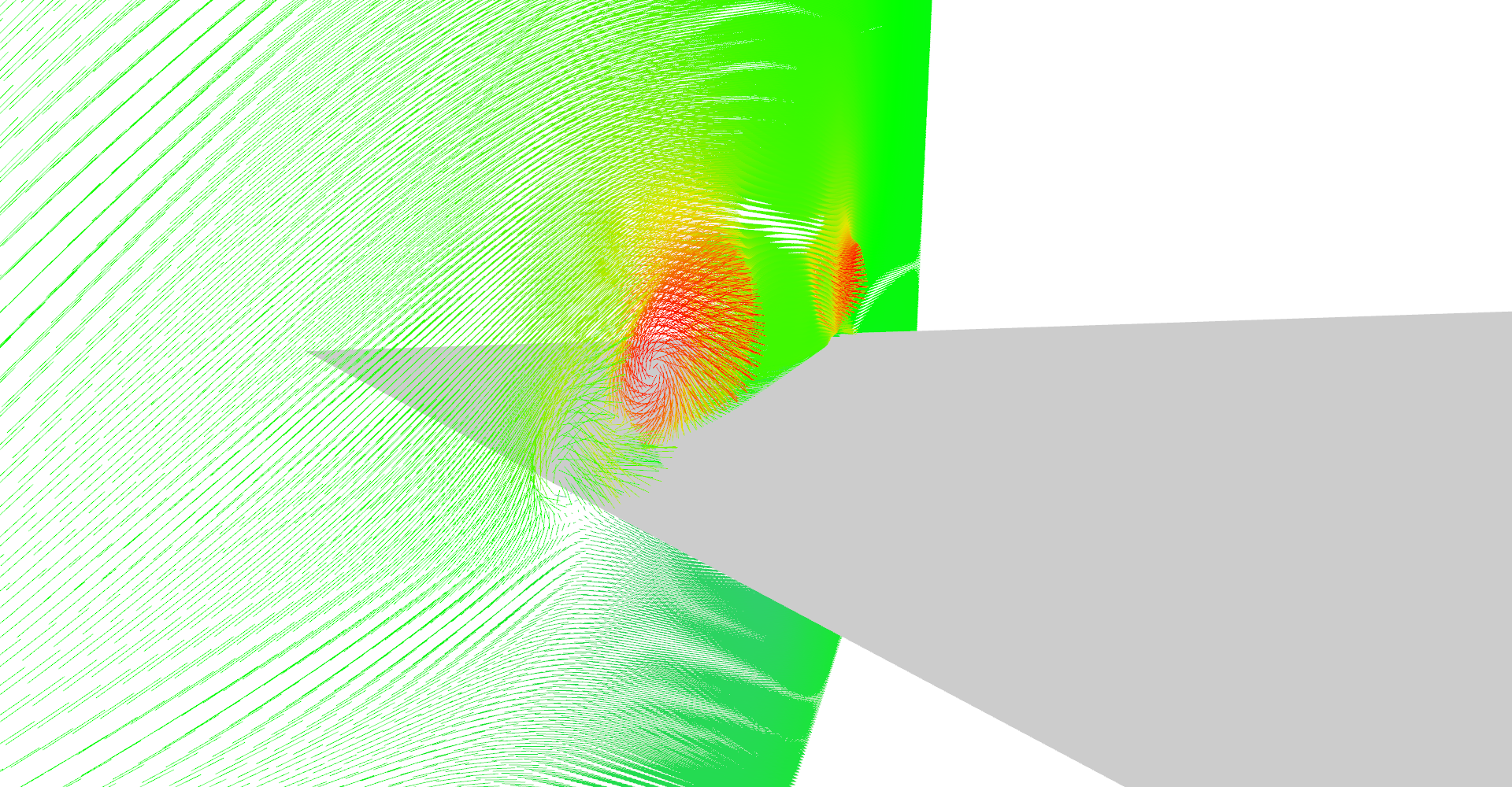
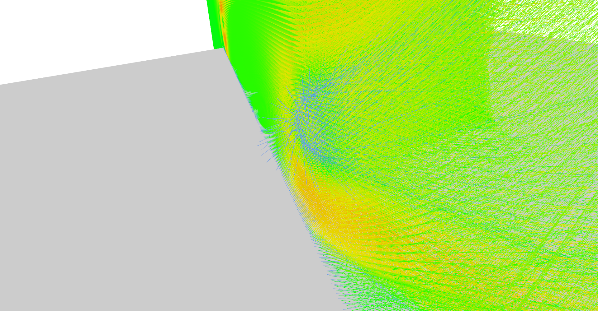
Results of this visualization are shown in Figure 4. As you can see, it is quite hard to "read" this visualization. Lines are not shaded which makes it very hard to see line orientation in space. This visualization is also ambiguous because you cannot tell correct length and direction of the line. The color scale helps to distinguish lines and line length. In the application itself the situation is a little bit better because you can move camera round and see line orientations and lengths more easily as well as smoothly move the plane with line glyphs on x-axis.
1
2
3
4
5
6
7
8
9
10
11
12
13
14
15
16
17
18
19
20
21
22
__global__ void glyphLinesKernel(float x, uint2 glyphsCount,
		float2 worldSize, float3* outVertices, float3* outColors) {

	uint id = __umul24(blockIdx.x, blockDim.x) + threadIdx.x;
	uint totalCount = __umul24(glyphsCount.x, glyphsCount.y);
	if (id >= totalCount) {
		return;
	}

	float y = (id % glyphsCount.x) * (worldSize.x / glyphsCount.x);
	float z = (id / glyphsCount.x) * (worldSize.y / glyphsCount.y);
	float4 vector = tex3D(vectorFieldTex, x, y, z);

	id *= 2;
	outVertices[id] = make_float3(x, y, z);
	outVertices[id + 1] = make_float3(x, y, z)
		+ normalize(make_float3(vector.x, vector.y, vector.z)) * vector.w;

	float4 color = tex1D(vectorMangitudeCtfTex, vector.w);
	outColors[id] = make_float3(color.x, color.y, color.z);
	outColors[id + 1] = make_float3(color.x, color.y, color.z);
}
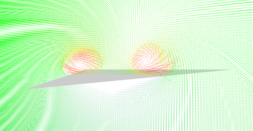
Line glyphs reveal two vortices above the sides of the wing. 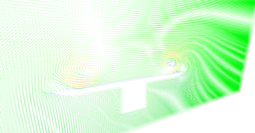
Line glyphs near the end of the wing - main vortices are weaker and you may notice very small secondary vortices. 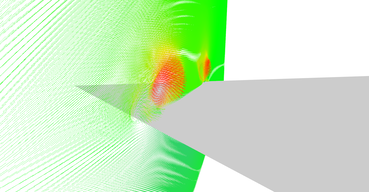
Detail on primary and secondary vortices above the sides of the wing. 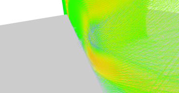
Detail on recirculation bubble where wind goes even backwards.
Performance of this visualization is very good because every CUDA thread has to compute just two points. Computation time for nearly any amount of glyphs is less than 20 ms which makes the exploration very responsive and intuitive.
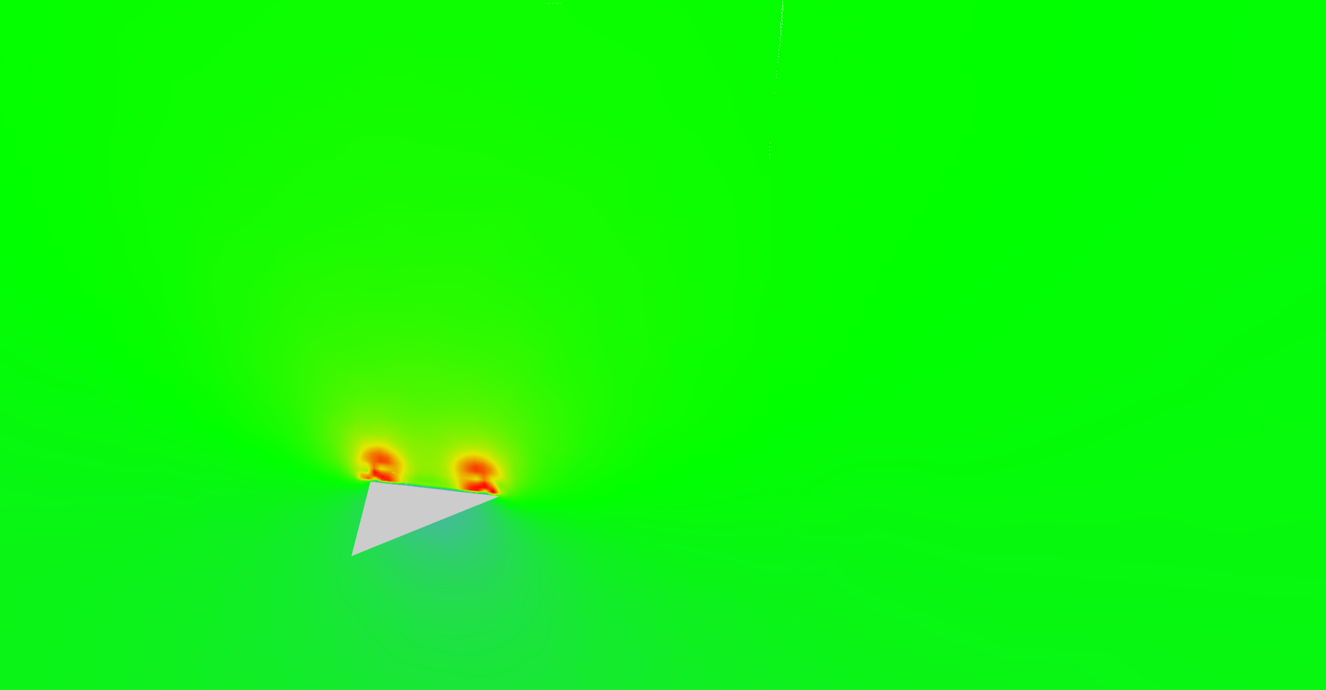
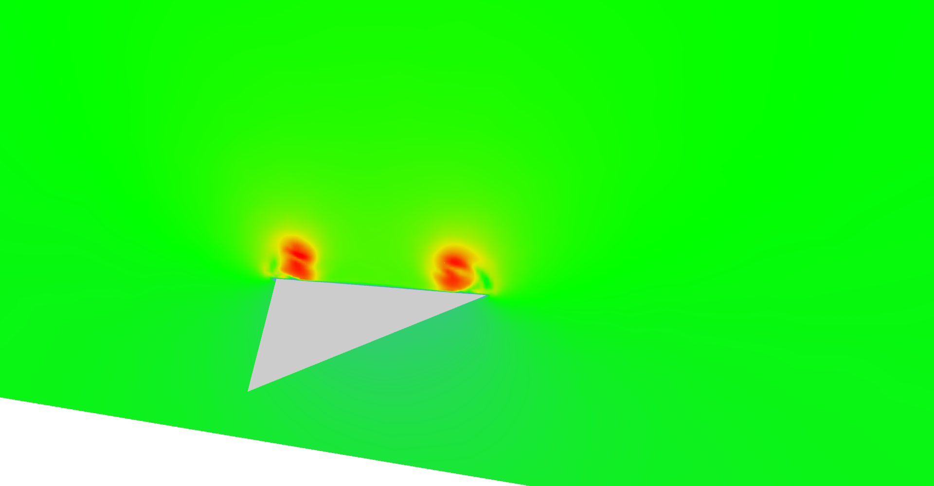
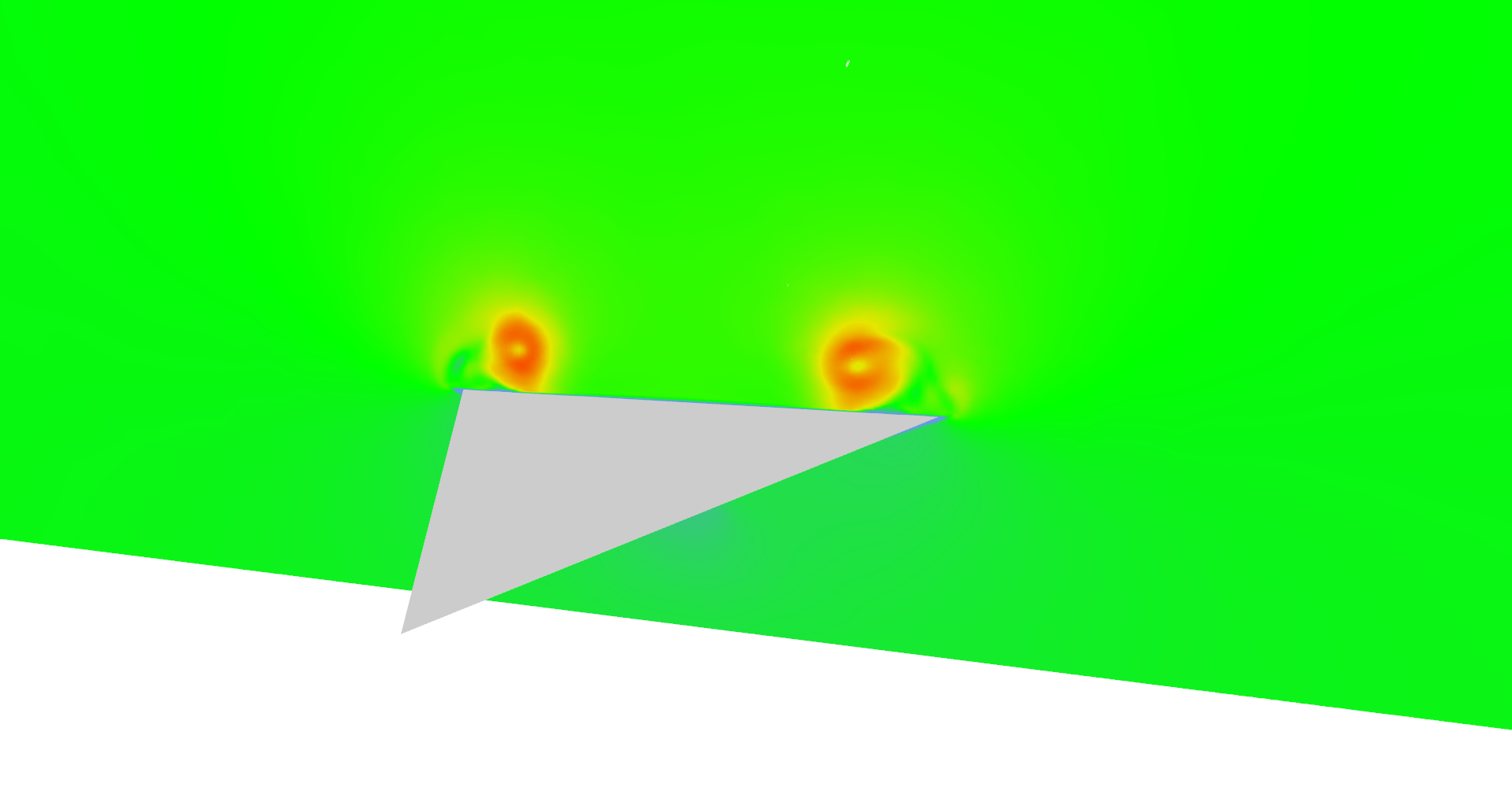
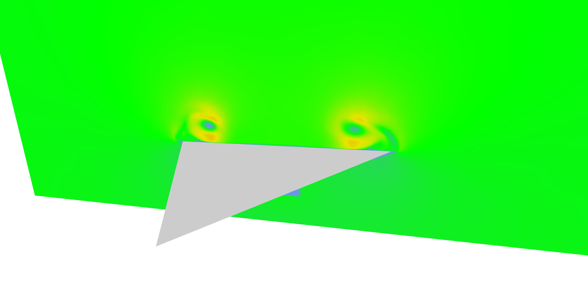
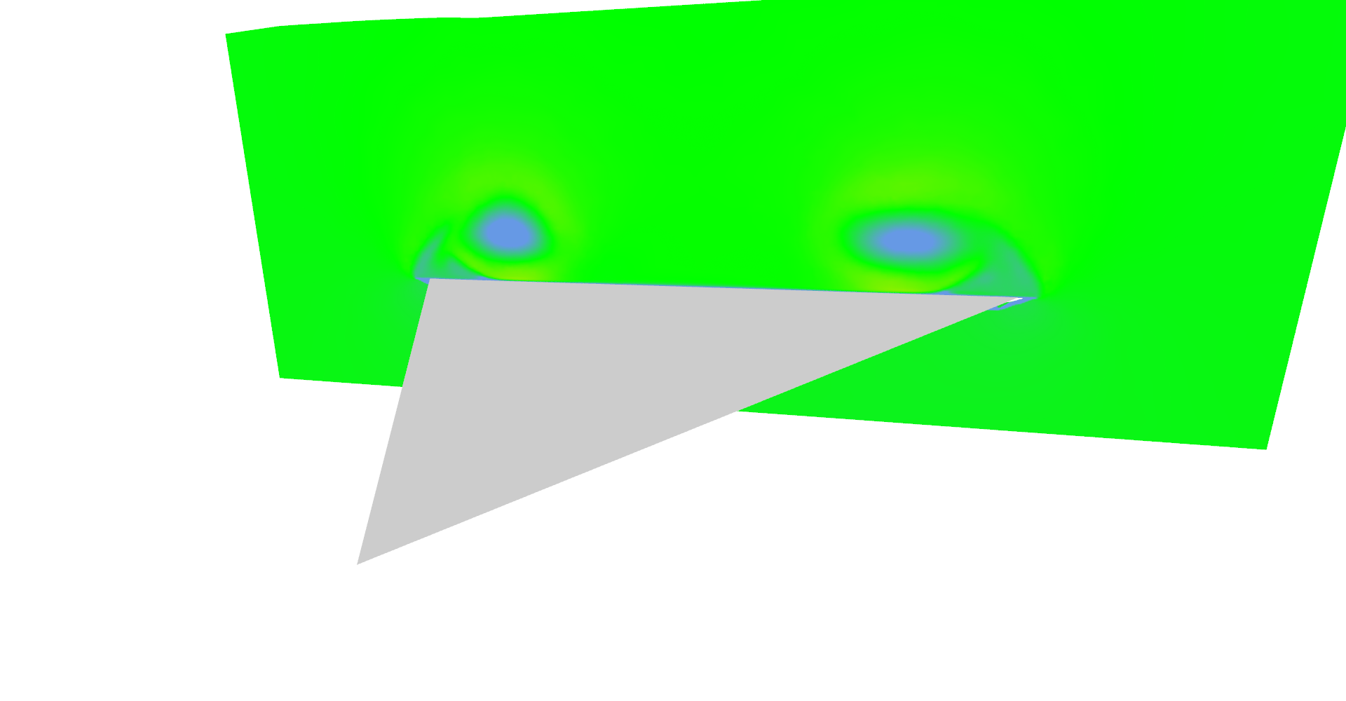
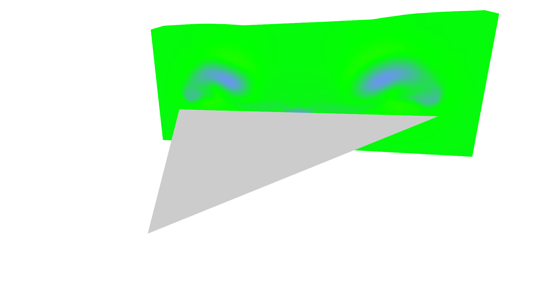
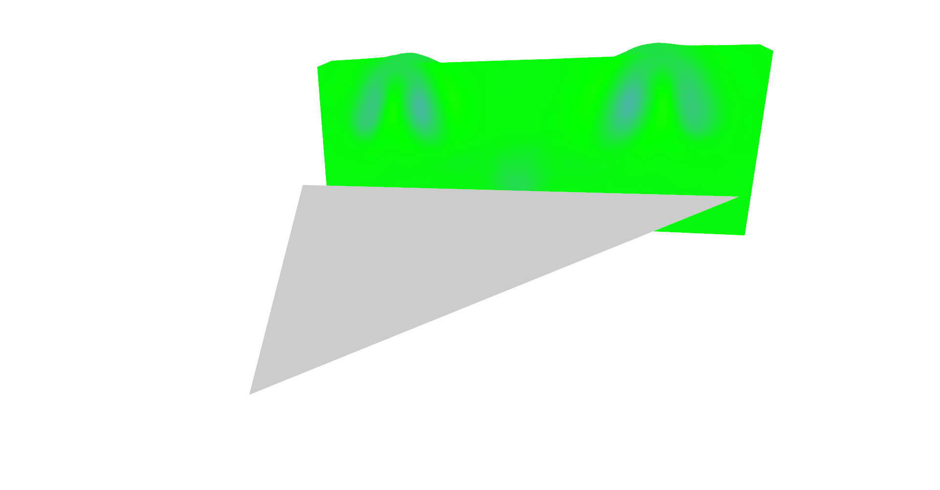
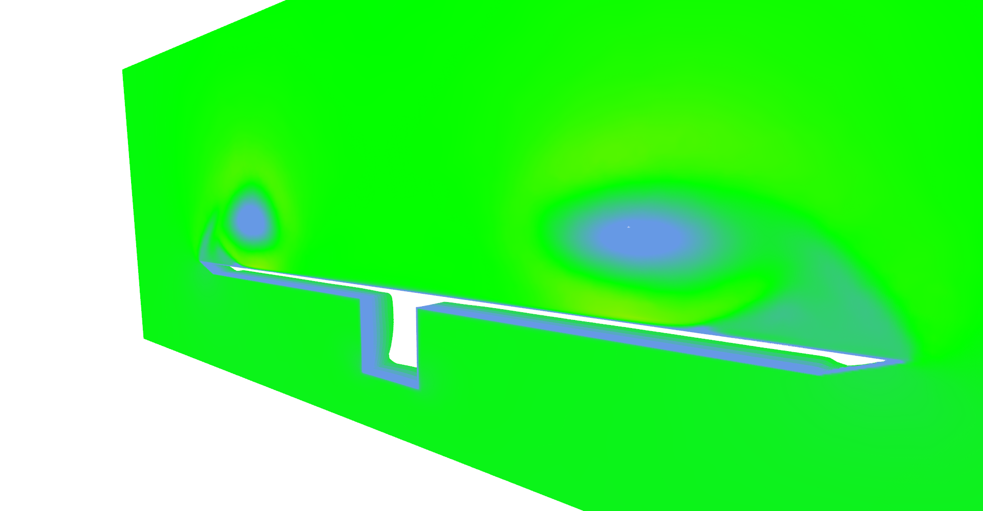
It is possible to set the number of glyph lines in a plane to very high numbers and create a solid wall as shown in Figure 5. This serves as a relatively nice visualization of vector magnitudes.
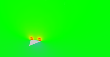
High density line glyphs plane effectively visualizing magnitude field. Plane is just behind the front of the wing. 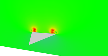
Vector field magnitudes near the middle of the wing. 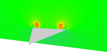
Vector field magnitudes near the middle of the wing. 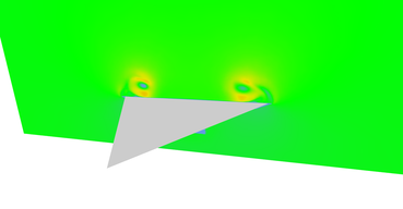
Vector field magnitudes near the end of the wing. 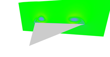
Vector field magnitudes near the end of the wing. 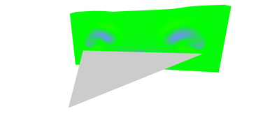
Vector field magnitudes just behind the wing. 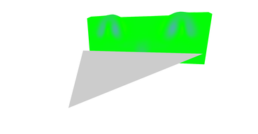
Vector field magnitudes further behind the wing. 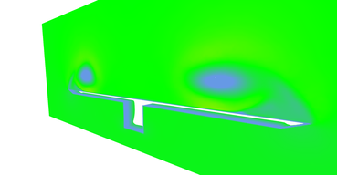
Vector field magnitudes near the end of the wing. Wing itself is not shown which reveals box under the wing. Notice that wind is slower near the surface of the wing.
Arrow glyphs for VF visualization#
As we saw, lines visualization is very ambiguous. Arrows help to remove those ambiguities. Orientation is distinguished by arrow itself and because arrow has triangular faces, it can be shaded according to light and thus seen in 3D more clearly.
Code listing 7 shows a (simplified) kernel for computation of arrow glyphs. An interesting fact about this kernel is that it computes vertices, normals and indices for all arrows. This makes the code quite lengthy but it also makes the computation and display blazingly fast. Thanks to usage of shared VBOs there is no CPU-GPU data transfer.
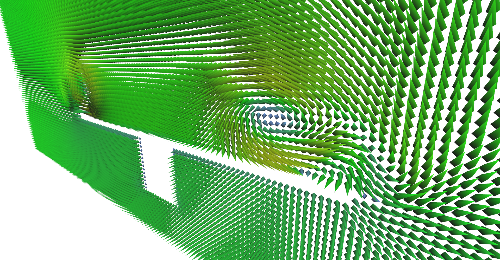
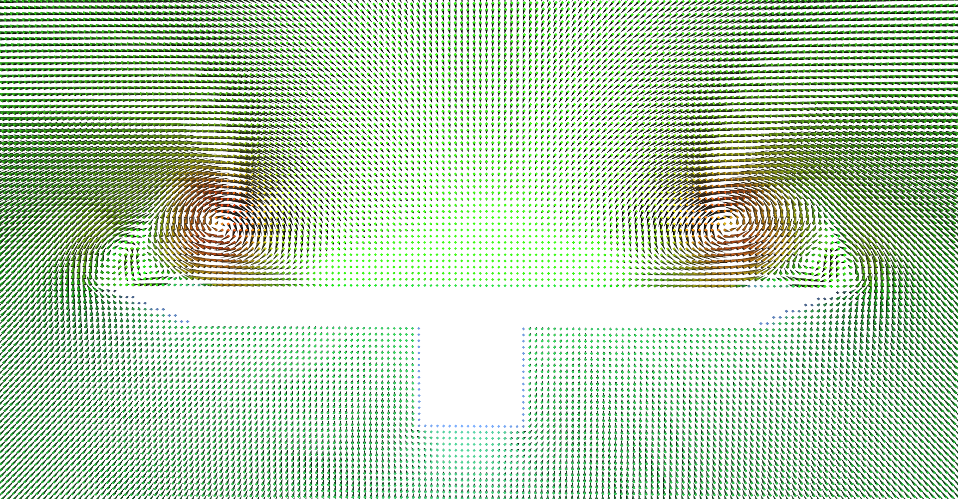
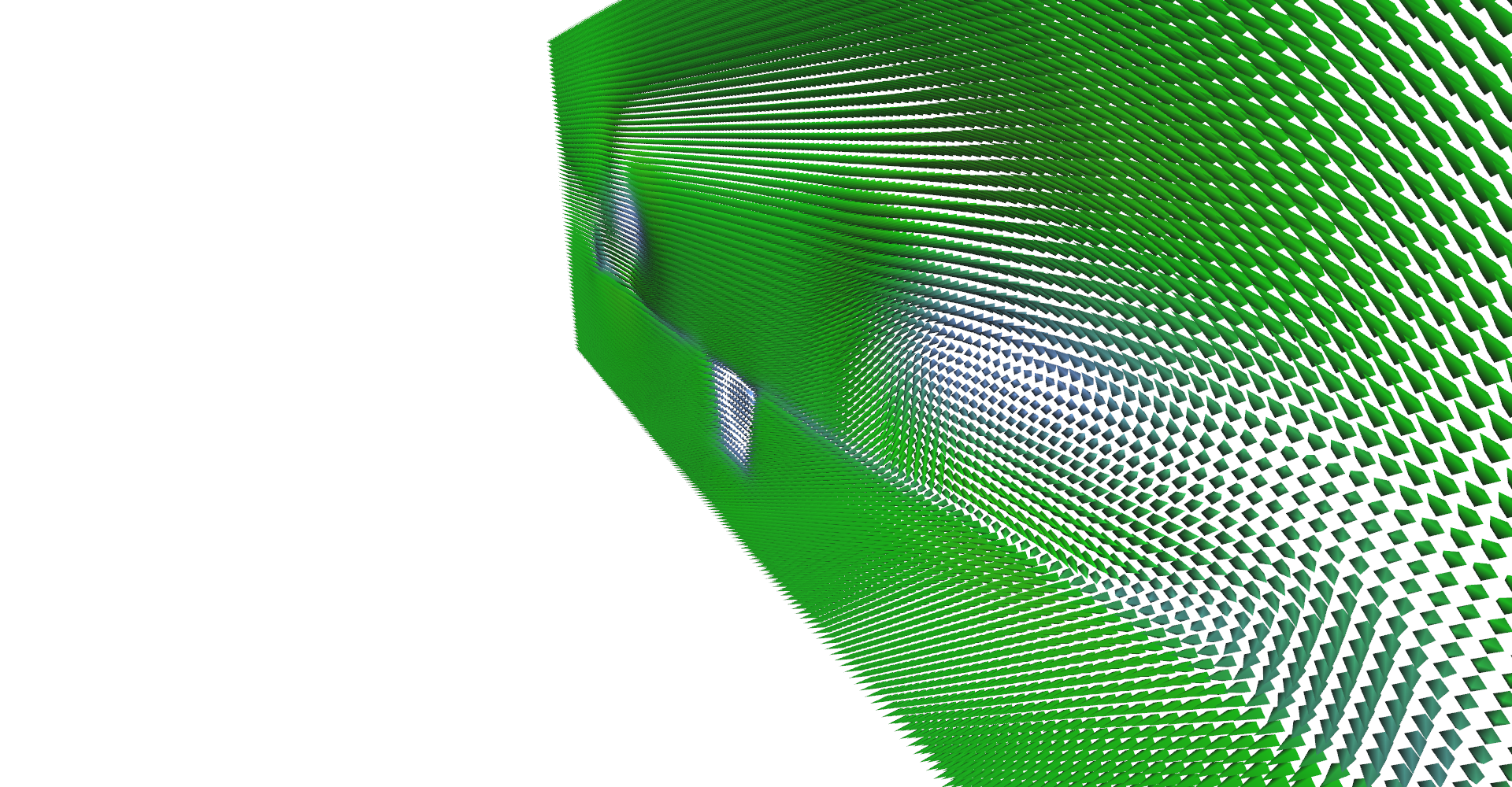
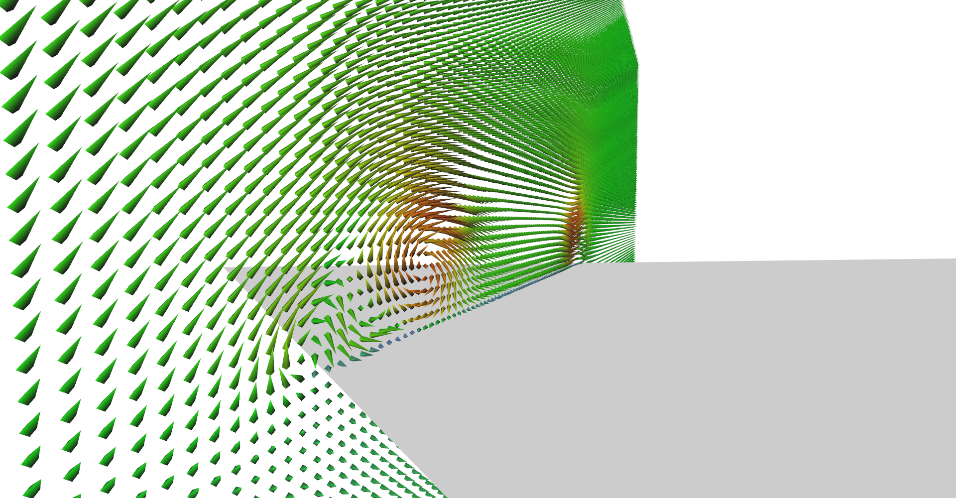
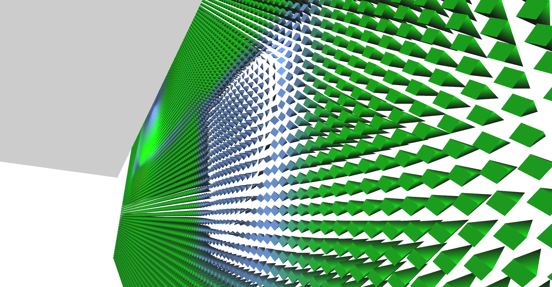
Arrows are much larger than lines thus, we need less of them and it makes the computation roughly 2x faster than lines (about 10 ms). Results of this visualization are shown in Figure 6. In the application it is possible to adjust density and size of arrow glyphs as well as smoothly move with the plane where glyphs are.
1
2
3
4
5
6
7
8
9
10
11
12
13
14
15
16
17
18
19
20
21
22
23
24
25
26
27
28
29
30
31
32
33
34
35
36
37
38
39
40
41
42
43
44
45
46
47
48
49
50
51
52
53
__global__ void glyphArrowsKernel(float x, uint2 glyphsCount,
		float2 worldSize, float3* outVertices, uint3* outFaces,
		float3* outVertexNormals, float3* outVertexColors) {

	uint id = __umul24(blockIdx.x, blockDim.x) + threadIdx.x;
	// ... same part as in lines kernel ...
	float4 vector = tex3D(vectorFieldTex, x, y, z);
	float3 forward = normalize(make_float3(vector.x, vector.y, vector.z));
	float3 xAxis = normalize(findPerpendicular(forward));
	float3 yAxis = normalize(cross(forward, xAxis));

	uint faceId = id * 6;
	uint vertId = id * 9;

	outFaces[faceId] = make_uint3(vertId, vertId + 1, vertId + 2);
	outFaces[faceId + 1] = make_uint3(vertId, vertId + 2, vertId + 3);
	outFaces[faceId + 2] = make_uint3(vertId, vertId + 3, vertId + 4);
	outFaces[faceId + 3] = make_uint3(vertId, vertId + 4, vertId + 1);
	outFaces[faceId + 4] = make_uint3(vertId + 5, vertId + 6, vertId + 7);
	outFaces[faceId + 5] = make_uint3(vertId + 5, vertId + 7, vertId + 8);

	id *= 9;
	outVertexNormals[id] = forward;
	outVertexNormals[id + 1] = xAxis;
	outVertexNormals[id + 2] = yAxis;
	outVertexNormals[id + 3] = -xAxis;
	outVertexNormals[id + 4] = -yAxis;
	forward *= -1;
	outVertexNormals[id + 5] = forward;
	outVertexNormals[id + 6] = forward;
	outVertexNormals[id + 7] = forward;
	outVertexNormals[id + 8] = forward;

	forward *= vector.w;
	xAxis *= 0.1;
	yAxis *= 0.1;

	outVertices[id] = position - forward;  // Forward was multiplied by -1.
	outVertices[id + 1] = position + xAxis;
	outVertices[id + 2] = position + yAxis;
	outVertices[id + 3] = position - xAxis;
	outVertices[id + 4] = position - yAxis;
	outVertices[id + 5] = position + xAxis;
	outVertices[id + 6] = position + yAxis;
	outVertices[id + 7] = position - xAxis;
	outVertices[id + 8] = position - yAxis;

	float4 color = tex1D(vectorMangitudeCtfTex, vector.w);
	float3 color3 = make_float3(color.x, color.y, color.z);
	for (int i = 0; i < 9; ++i) {
		outVertexColors[id + i] = color3;
	}
}
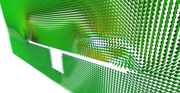
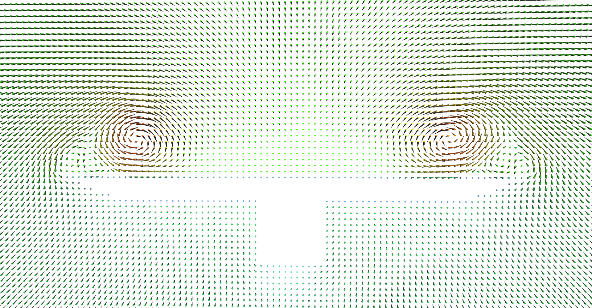
Vector field visualization using arrow glyphs near the end of the wing. 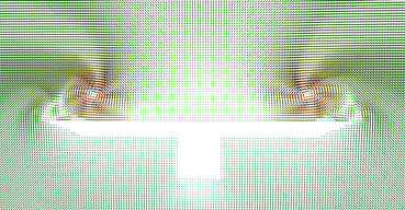
Front view of glyphs plane going through the middle of the wing. Notice secondary vortices under the primary ones. 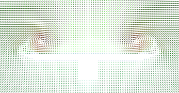
Lower density of arrow glyphs. 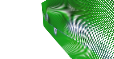
Glyphs plane just behind the delta-wing. 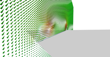
Another view on glyph plane from the back. 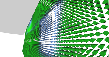
Detail on the area behind the aerodynamic box of the wing where air is going in the opposite direction (the box is not shown).
Line vs. arrow glyphs#
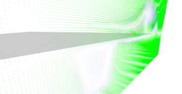
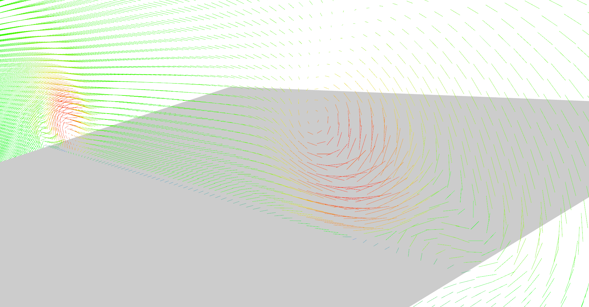
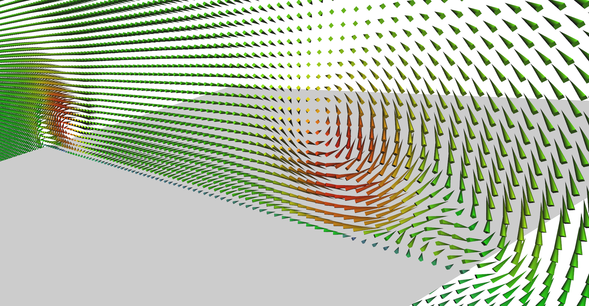
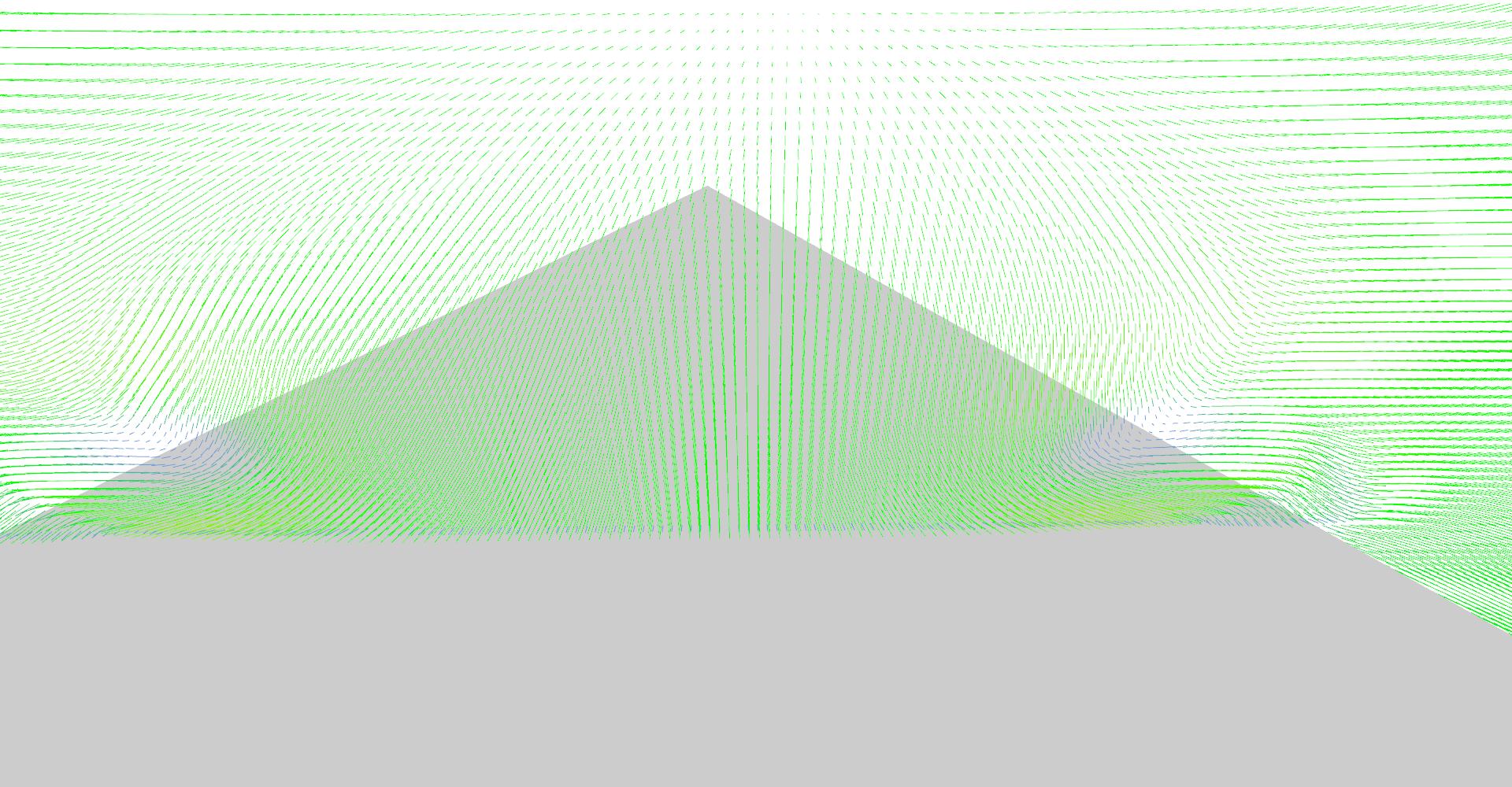
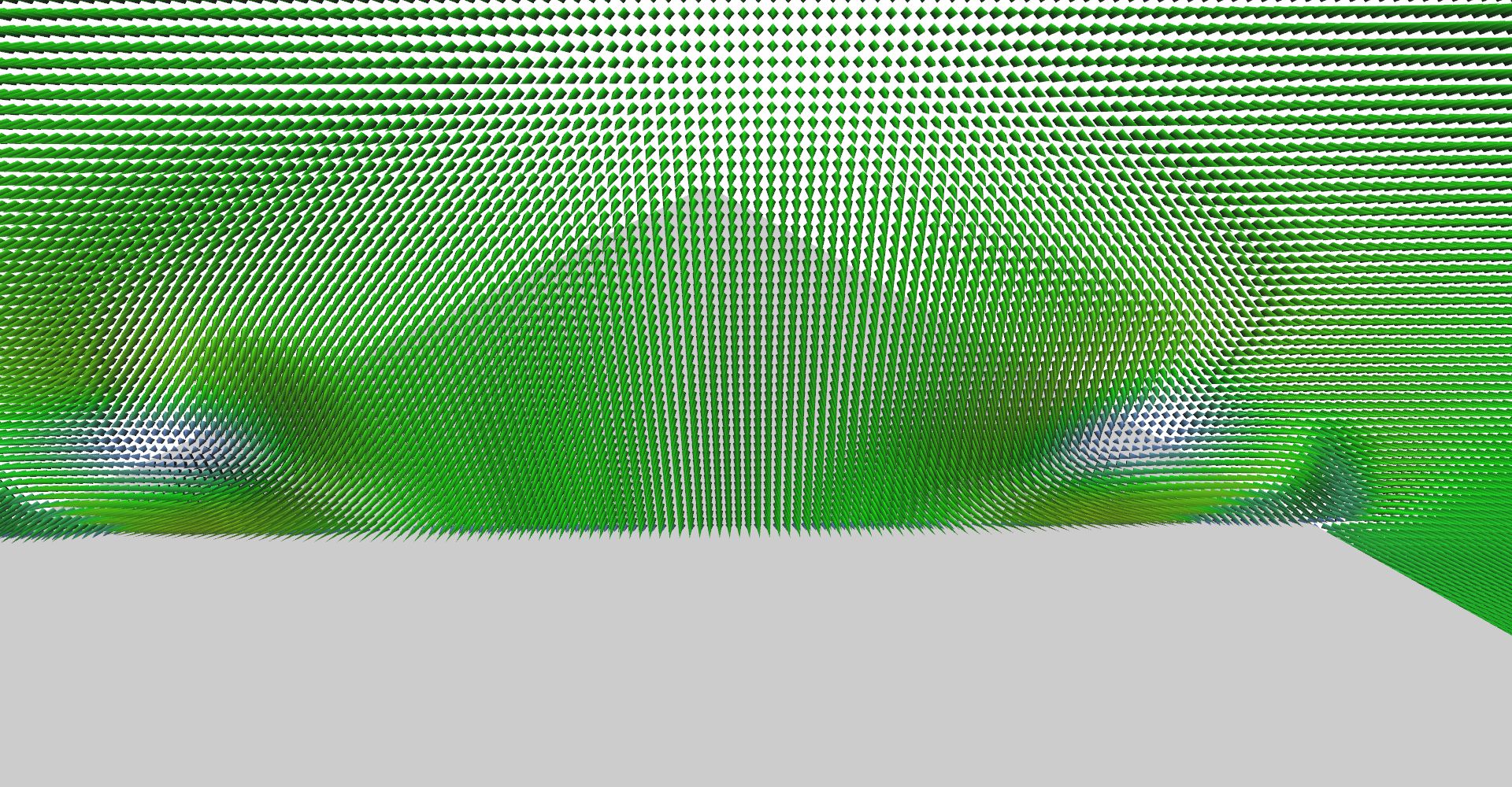
Figure 7 shows a side-by-side comparison of line and arrow glyphs. This nicely shows that arrows do a much better job in vector field visualization. However, there are better techniques how to visualize vector fields which are discussed in the following sections.
Line vs. arrow glyphs (pair 1, lines). 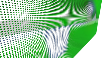
Line vs. arrow glyphs (pair 1, arrows). 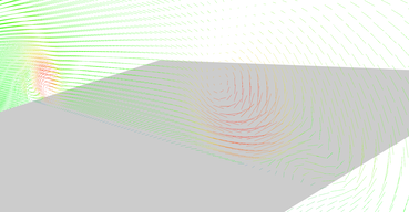
Line vs. arrow glyphs (pair 2, lines). 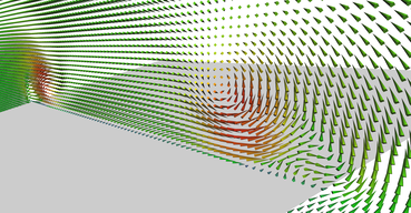
Line vs. arrow glyphs (pair 2, arrows). 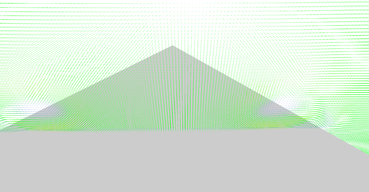
Line vs. arrow glyphs (pair 3, lines). 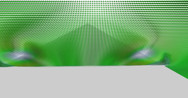
Line vs. arrow glyphs (pair 3, arrows).
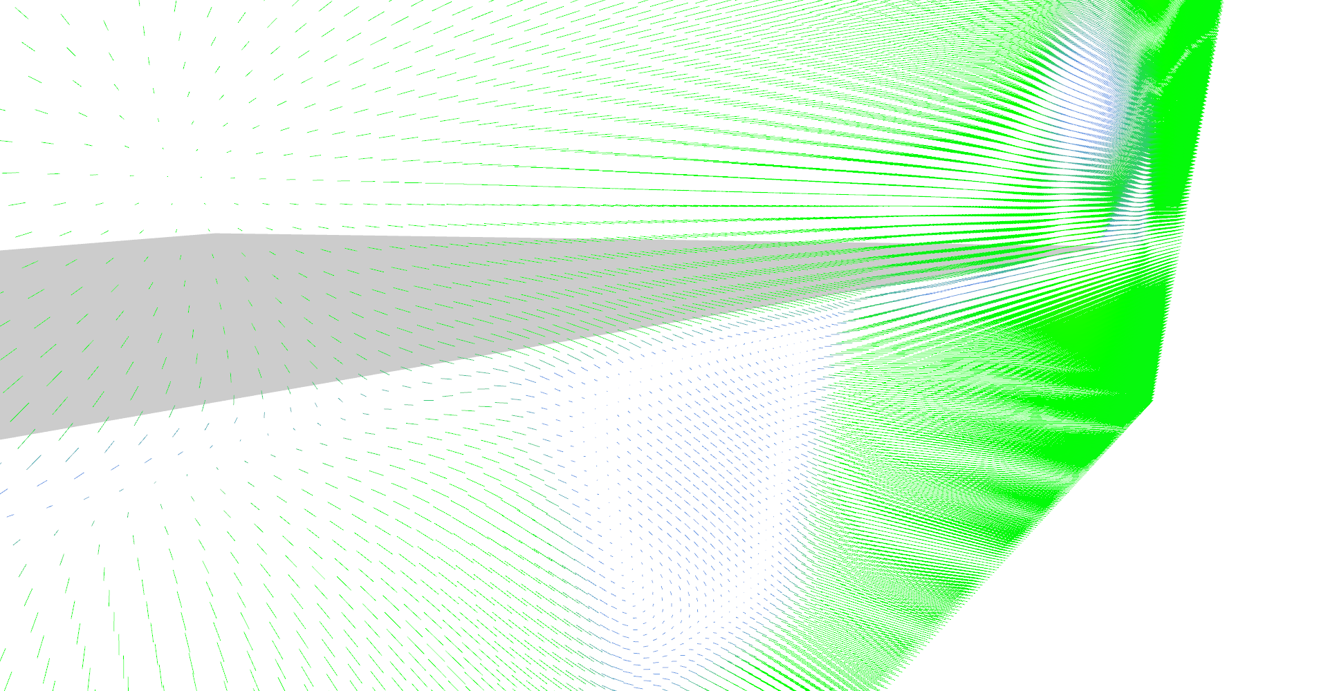
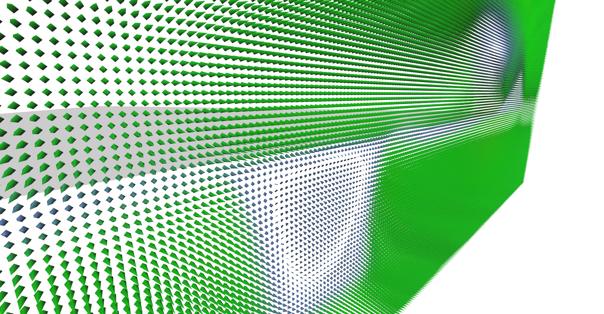
3. Vector field integrators for stream line visualization#
Before we jump into visualization techniques using stream lines and stream surfaces I would like to mention implementation details of used integrators.
A stream line is a trajectory of a mass-less particle in a vector field. Integrators are used to simulate this trajectory by moving a particle according to the vector field orientation and magnitude by discrete steps. Step size determines how precise this process will be. A large step size will cause more error but a smaller step size will take more time to compute desired length of the curve.
Euler integrator#
The simplest integrator uses Euler method for integration.
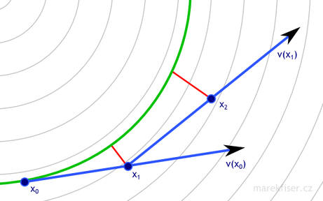
The integration step is computed based on current position and vector field value at that position (Equation 1).
Figure 8 shows a comparison of integration with step dt = 0.5 and dt = 0.25.
You can see that a shorter time-step results in better results (less error - marked as red lines).
xn+1 = xn + dt ∙ v(xn) + O(dt2), where xnis current position,xn+1is next position,dtis time step,v(xn)is vector field at position xn, andO(dt2)is error.
dt = 0.5 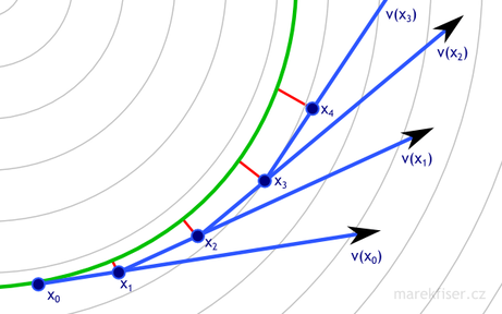
dt = 0.25
Implementation is literally two lines of code (Code listing 8) and that's the primary reason why I implemented it. However, the down side is that local error (error per step) is proportional to the square of the step size, and the global error (error at a given time) is proportional to the step size.
1
2
3
4
__device__ double4 eulerIntegrate(double3 pos, double dt) {
	float4 v = tex3D(vectorFieldTex, (float)pos.x, (float)pos.y, (float)pos.z);
	return make_double4(dt * v.x, dt * v.y, dt * v.z, v.w);
}
Runge–Kutta 4 integrator#
First, I thought that the Euler integrator would be enough since CUDA is fast and I can set step size very small. Later in the project it turned out that step size is important for performance and also that lowering step size does not reduce error too much.
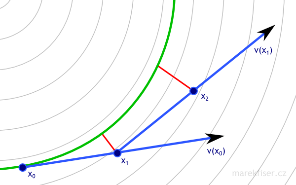
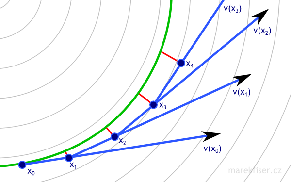
I decided to implement a better integrator called Runge–Kutta 4 (Code listing 9). In short, the integrator queries vector field in four cleverly chosen positions and combines results to one step. Equation 6 shows exact equations of integration step and Figure 9 shows the situation visually (please note that this figure was done by hand and actual result could be slightly different). The error of RK4 integrator is smaller by an order of magnitude compared to Euler and for some special cases (like circular vector field) might have even no error. For more details on how this integrator works please see the article on Wikipedia about Runge–Kutta methods.
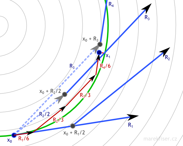 Figure 9: One step of RK4 integration with dt = 1.
Vector field is shown as thin gray lines, green curve represents ground truth,
blue arrows are vectors used in computation of RK4 integration, dark red arrows are actual RK4 steps,
and small bright red line represents error.
Note that RK4 has much smaller error than Euler (Figure 8) even for much bigger time step.
Figure 9: One step of RK4 integration with dt = 1.
Vector field is shown as thin gray lines, green curve represents ground truth,
blue arrows are vectors used in computation of RK4 integration, dark red arrows are actual RK4 steps,
and small bright red line represents error.
Note that RK4 has much smaller error than Euler (Figure 8) even for much bigger time step.k1 = dt ∙ v(xn)k2 = dt ∙ v(xn + k1/2)k3 = dt ∙ v(xn + k2/2)k4 = dt ∙ v(xn + k3)xn+1 = xn + k1/6 + k2/3 + k3/3 + k4/6 + O(dt5), where xnis current position,xn+1is next position,dtis time step,v(x)is vector field at position x, andO(dt5)is error.
The big advantage of the Runge–Kutta integrator is much lower error of integration but it requires more computation power.
You can see that Euler's method for dt=0.5 (Figure 8) has larger error than RK4 method for 4-times larger time step dt = 1 (Figure 9).
section Comparison of Euler and RK4 integrators compares both integrators and shows the performance comparison (RK4 is about 4x slower than Euler).
In all the following sections the Runge–Kutta 4 integrator is used.
1
2
3
4
5
6
7
8
9
10
11
12
13
14
15
16
17
18
__device__ double4 rk4Integrate(double3 pos, double dt) {
	double dtHalf = dt * 0.5;

	float4 k1 = tex3D(vectorFieldTex, (float)pos.x, (float)pos.y, (float)pos.z);
	float4 k2 = tex3D(vectorFieldTex, (float)(pos.x + dtHalf * k1.x),
		(float)(pos.y + dtHalf * k1.y), (float)(pos.z + dtHalf * k1.z));
	float4 k3 = tex3D(vectorFieldTex, (float)(pos.x + dtHalf * k2.x),
		(float)(pos.y + dtHalf * k2.y), (float)(pos.z + dtHalf * k2.z));
	float4 k4 = tex3D(vectorFieldTex, (float)(pos.x + dt * k3.x),
		(float)(pos.y + dt * k3.y), (float)(pos.z + dt * k3.z));

	double dtSixth = dt / 6.0;
	return make_double4(
		dtSixth * (k1.x + 2.0 * ((double)k2.x + k3.x) + k4.x),
		dtSixth * (k1.y + 2.0 * ((double)k2.y + k3.y) + k4.y),
		dtSixth * (k1.z + 2.0 * ((double)k2.z + k3.z) + k4.z),
		(k1.w + 2.0 * ((double)k2.w + k3.w) + k4.w) / 6.0);
}
4. Visualization using stream lines and stream tubes#
This section shows results of stream line visualization of delta-wing vector field data set. This type of visualization will provide much better understanding of the data than glyphs described in section 2: Visualization using glyphs.
Stream lines#
As mentioned in section 3: Vector field integrators for stream line visualization, a stream line is a trajectory of a mass-less particle in a vector field. Once we have an integrator, visualization is straightforward. Seed the stream line somewhere in the vector field, compute points at discrete time steps and connect them to a line. The color of the line segment represents the vector magnitude - in our case speed of the air.
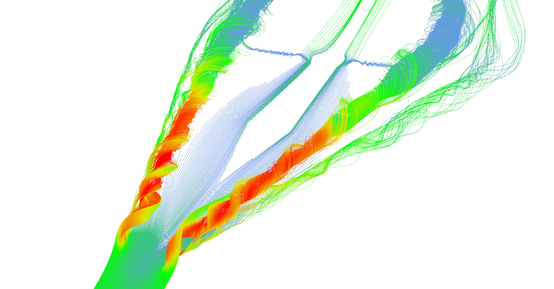
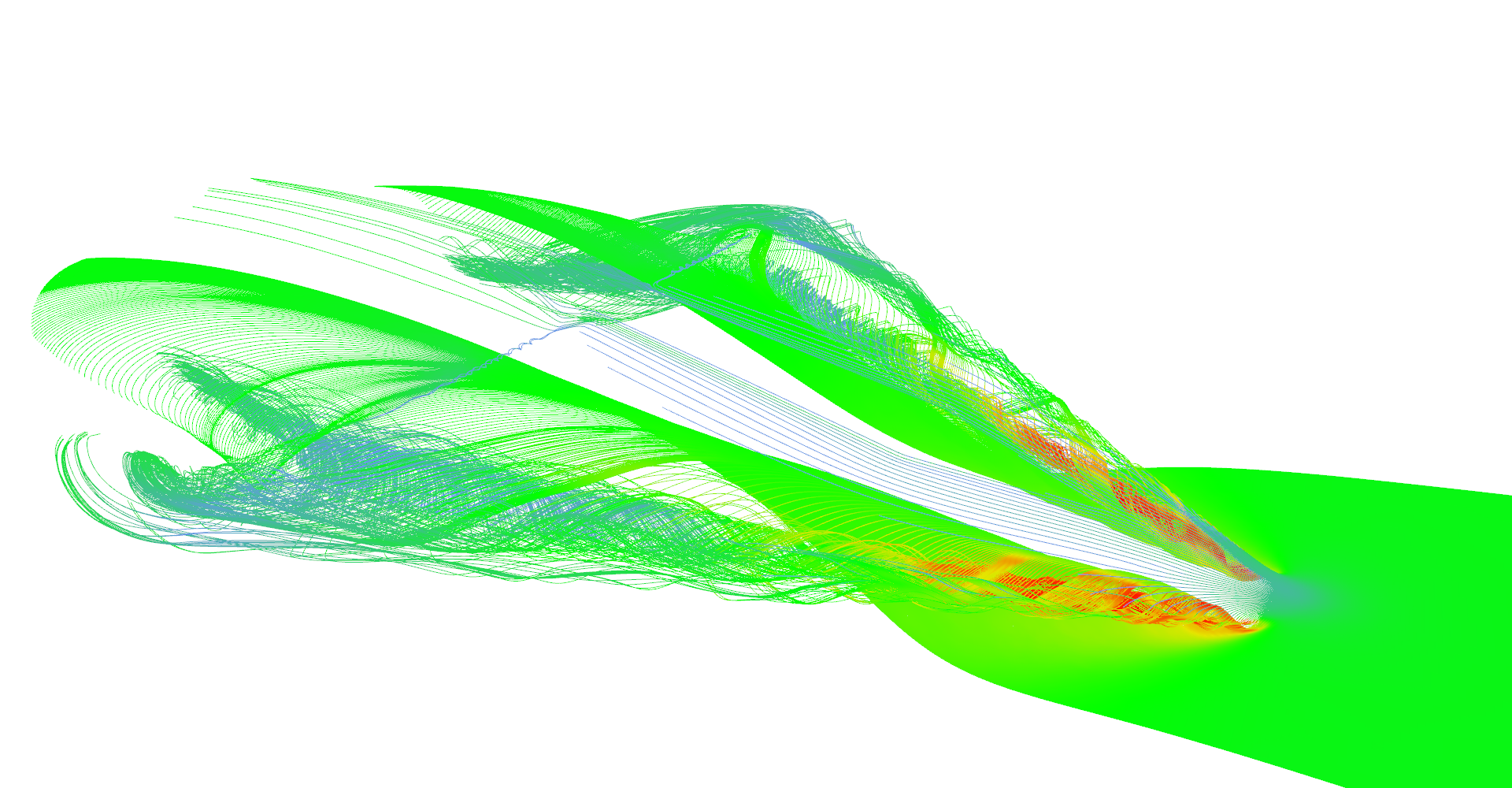
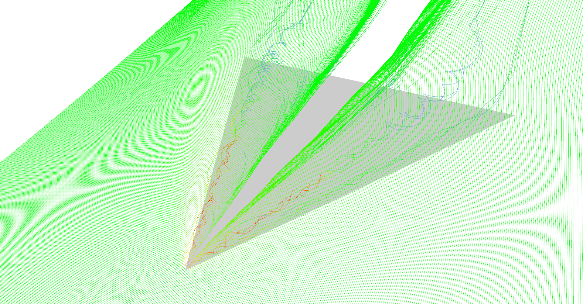
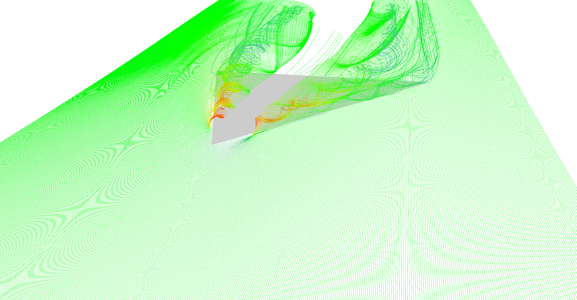
The only problem is where to seed the line, there are many possible approaches to this. I decided to seed stream lines on the straight line. User can interactively move this seed-line to explore the vector field.
The first image in Figure 10 shows all features of the delta wing dataset. There are primary and secondary vortices rolling above the edges of the wing as well as turbulences behind the wing edge.
Code listing 10 shows a simplified kernel for evaluation of an array of stream lines. Every stream line is evaluated on a separate thread so the true benefit comes with evaluation of more than one line.
Notice that kernel integrates the stream line in double precision but saves the result in single precision.
Also, to save GPU memory there is a parameter called geometrySampling which specifies how many integration samples per emitted geometry sample.
If geometrySampling is set to 1, every step is emitted but for number 2 only every second point is emitted.
This allows having very short integration step for great precision while being able to save results in limited GPU memory.
1
2
3
4
5
6
7
8
9
10
11
12
13
14
15
16
17
18
19
20
21
22
23
24
25
26
27
28
29
30
31
32
33
34
35
36
37
38
39
40
41
42
43
44
45
46
47
48
49
50
51
__global__ void computeStreamlinesLineKernel(float3* seeds,
			uint seedsCount, double dt, uint maxSteps,
			cudaExtent volumeSize, uint geometrySampling, float3* outVertices,
			uint* outComputedSteps, float3* outVertexColors) {

		uint id = __umul24(blockIdx.x, blockDim.x) + threadIdx.x;
		if (id >= seedsCount) {
			return;
		}

		uint outIndex = id * (maxSteps / geometrySampling + 1);
		// Integration is double precision.
		double3 position = make_double3(seeds[id].x, seeds[id].y, seeds[id].z);

		outVertices[outIndex].x = (float)position.x;
		outVertices[outIndex].y = (float)position.y;
		outVertices[outIndex].z = (float)position.z;
		++outIndex;

		uint geometryStep = geometrySampling;
		uint step = 1;
		for (; step < maxSteps; ++step) {
			if (position.x < 0 || position.y < 0 || position.z < 0
					|| position.x > volumeSize.width
					|| position.y > volumeSize.height
					|| position.z > volumeSize.depth) {
				break;
			}

			double4 dv = rk4Integrate(position, dt);
			position.x += dv.x;
			position.y += dv.y;
			position.z += dv.z;

			--geometryStep;
			if (geometryStep == 0) {
				geometryStep = geometrySampling;

				outVertices[outIndex].x = (float)position.x;
				outVertices[outIndex].y = (float)position.y;
				outVertices[outIndex].z = (float)position.z;
				setColorTo(outVertexColors[outIndex - 1], (float)dv.w);
				++outIndex;
			}
		}

		// Color of the last line point.
		outVertexColors[outIndex - 1] - outVertexColors[outIndex - 2];
		// Save the number of computed line segments.
		outComputedSteps[id] = step / geometrySampling;
	}
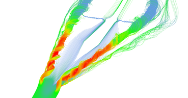
Stream lines seeded at very small area near the tip of the wing. Primary and secondary vortices are nicely visible as well as air moving sideways behind the edge of the wing. 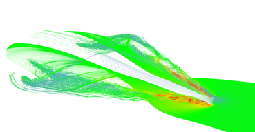
Slightly different setup as previous image. 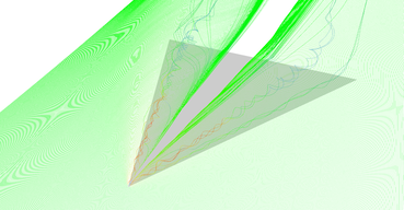
Stream lines seeded at long line in front of the wing. 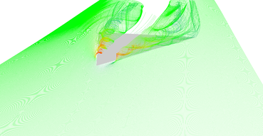
Slightly different setup as previous image.
Stream tubes#
Stream lines visualization suffers from very similar problems with ambiguity as line glyphs. It is hard to see the actual position of the line in space in the still image. The fact that there are many lines seeded in a straight line helps to imagine orientation but sometimes it is still hard. In the application, you can freely rotate the scene and discover the orientation but results of visualization are usually published as still images.
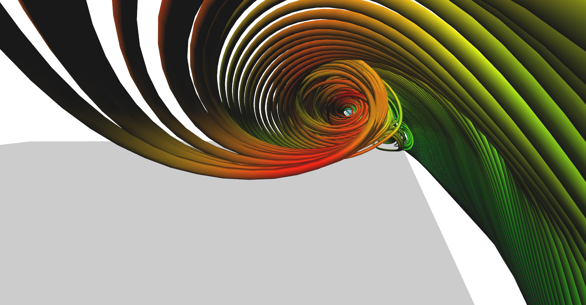
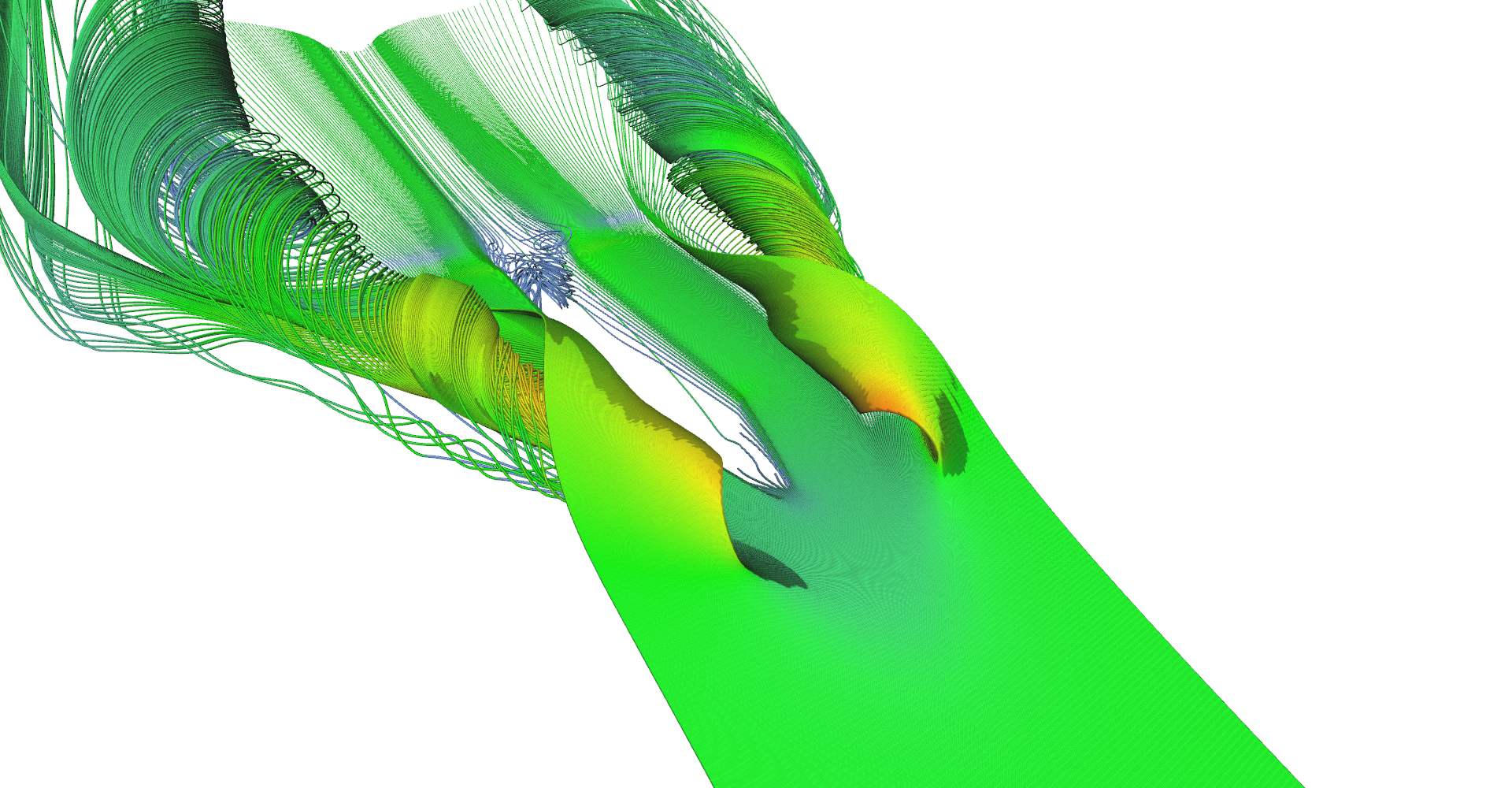
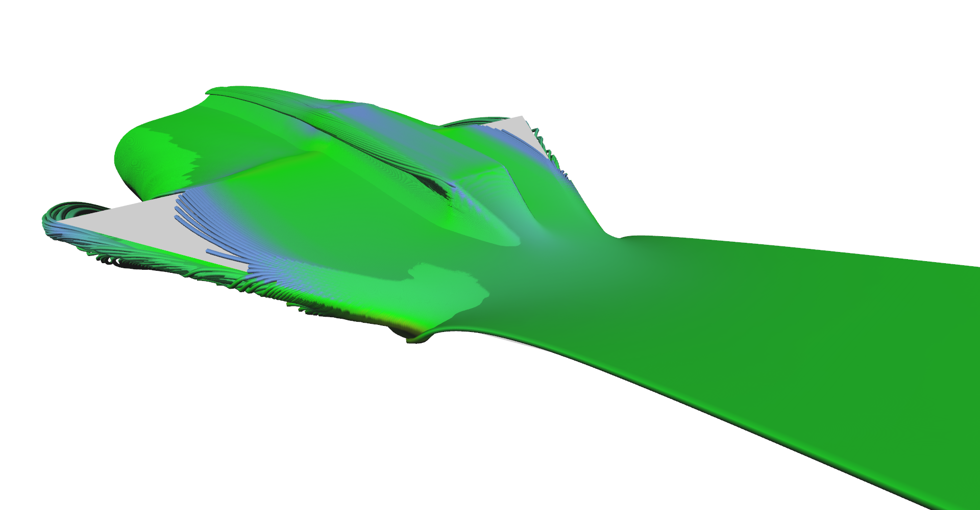
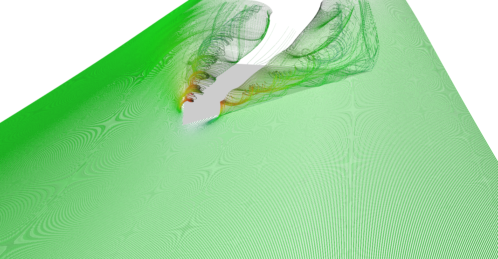
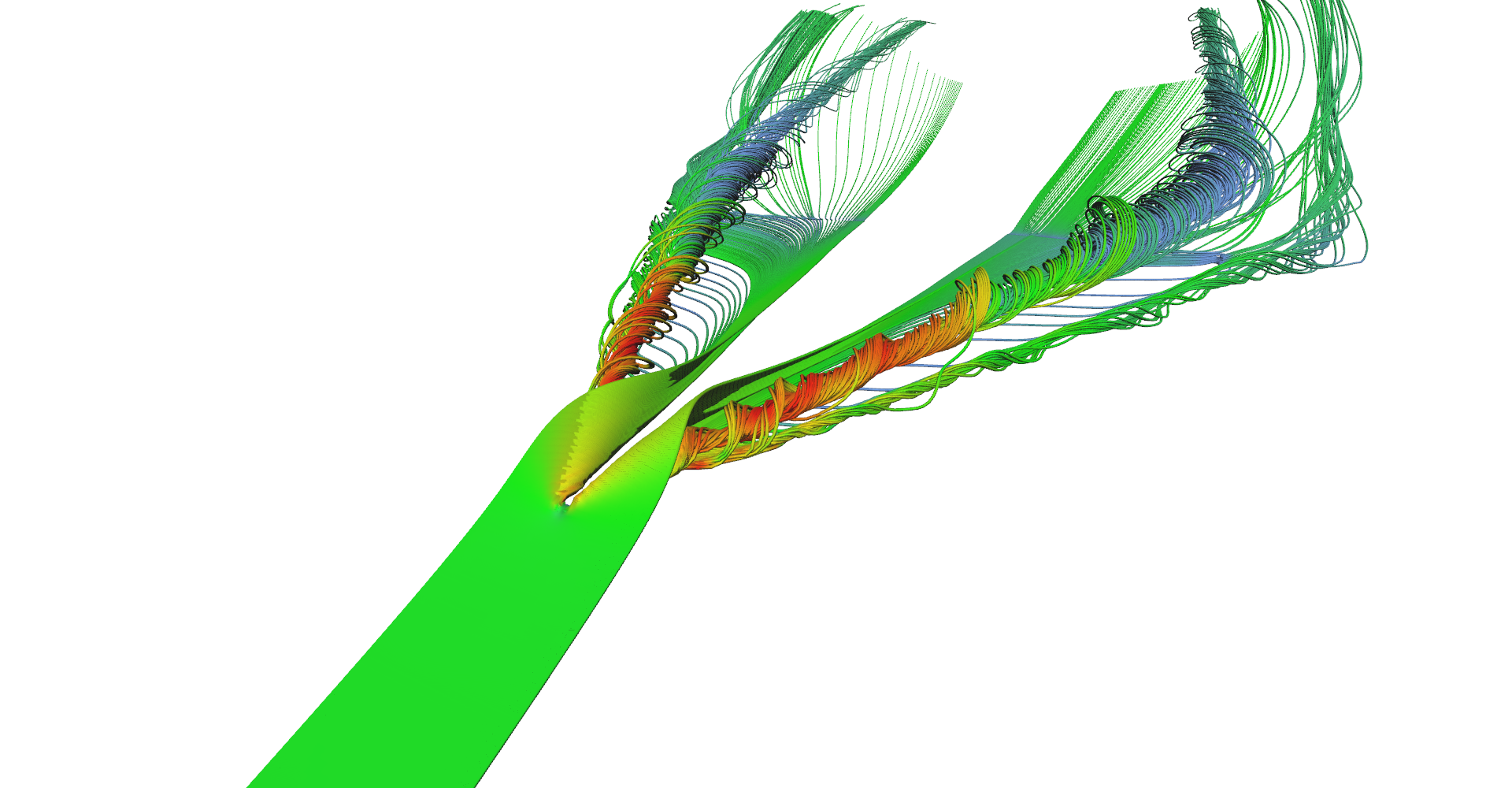
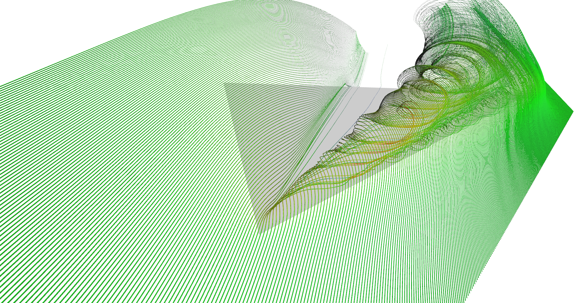
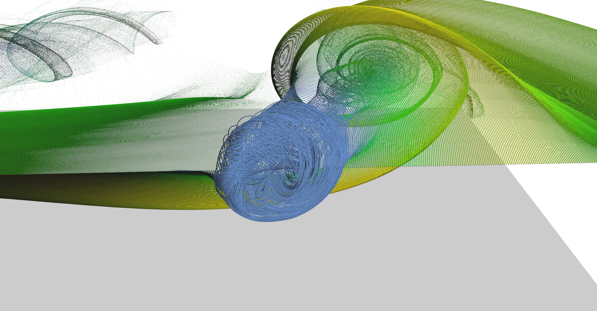
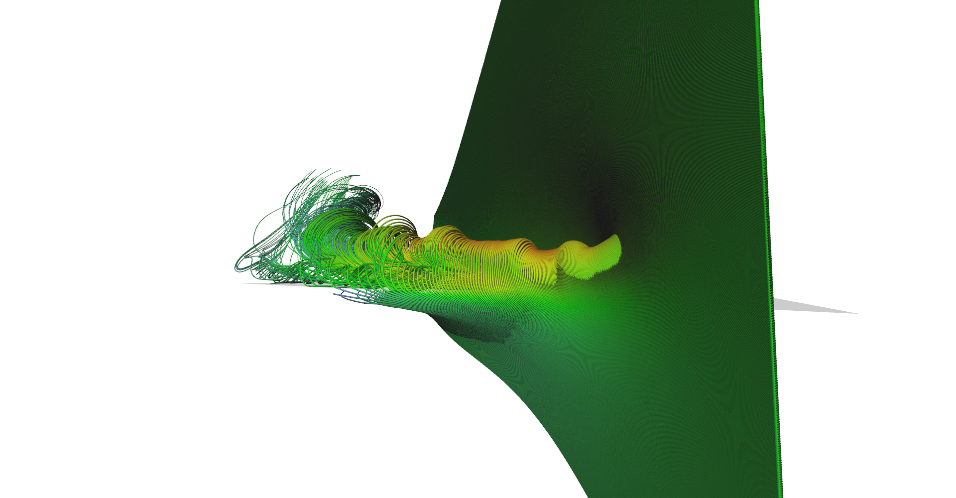
The trick is to inflate thin lines with some volume and create tubes, stream-tubes. Tubes can be shaded and if there are enough of them close to each other they form a nicely shaded surface. Figure 11 shows many images of this type of visualization.
CUDA kernel for computation of stream tubes is very similar to stream lines. The only difference is that we no longer save the position itself but we "extrude" a tube around it. Tube extrusion is done in the plane given by a vector from the vector field. Tube is constructed only with 5 sides to save as much GPU memory as possible. This sounds like very few but combined with smooth shading it is enough. This will ensure that the tube will nicely follow the stream line in any direction. Code for generation of tube geometry is shown in Code listing 11.
1
2
3
4
5
6
7
8
9
10
11
12
13
14
15
16
17
18
19
20
21
22
23
24
25
26
27
28
29
30
31
32
33
34
35
36
37
38
39
40
41
42
43
44
45
46
47
48
49
50
51
__device__ void createTubeBaseVertices(float3 pos, float3 v,
		float radius, uint baseIndex, float3 color,
		float3* outVetrices, float3* outNormals, float3* outColors) {

	float3 xAxis = normalize(findPerpendicular(v));
	float3 yAxis = normalize(cross(v, xAxis));

	// x * cos(0) + y * sin(0)
	outNormals[baseIndex] = xAxis;
	outVetrices[baseIndex] = pos + xAxis * radius;
	outColors[baseIndex] = color;
	++baseIndex;

	// x * cos(72) + y * sin(72)
	v = 0.3090f * xAxis + 0.9511f * yAxis;
	outNormals[baseIndex] = v;
	outVetrices[baseIndex] = pos + v * radius;
	outColors[baseIndex] = color;
	++baseIndex;

	// x * cos(144) + y * sin(144)
	v = -0.8090f * xAxis + 0.5878f * yAxis;
	outNormals[baseIndex] = v;
	outVetrices[baseIndex] = pos + v * radius;
	outColors[baseIndex] = color;
	++baseIndex;

	// x * cos(216) + y * sin(216)
	v = -0.8090f * xAxis - 0.5878f * yAxis;
	outNormals[baseIndex] = v;
	outVetrices[baseIndex] = pos + v * radius;
	outColors[baseIndex] = color;
	++baseIndex;

	// x * cos(288) + y * sin(288)
	v = 0.3090f * xAxis - 0.9511f * yAxis;
	outNormals[baseIndex] = v;
	outVetrices[baseIndex] = pos + v * radius;
	outColors[baseIndex] = color;
}

__device__ void createTubeIndices(uint vertexBaseId, uint baseFaceId, uint3* outFaces) {

	for (uint i = 0; i < 5; ++i) {
		uint iNext = (i + 1) % 5;
		outFaces[baseFaceId++] = make_uint3(vertexBaseId + i,
			vertexBaseId + iNext, vertexBaseId - 5 + iNext);
		outFaces[baseFaceId++] = make_uint3(vertexBaseId + i,
			vertexBaseId - 5 + i, vertexBaseId - 5 + iNext);
	}
}
Stream tubes showing the main features of the delta-wing dataset - primary and secondary vortices and air going sideways behind the back edge of the wing. 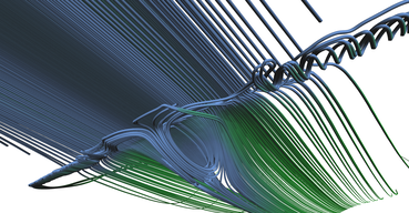
Detail on the back of the wing from the bottom. You can clearly see the vortex behind the box on the wing (the wing and the box are not shown). 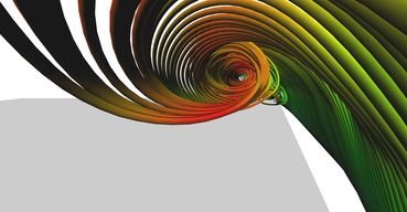
Detail of the primary vortex. 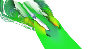
Another visualization of the datasets using stream-tubes. 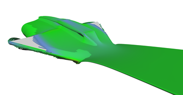
Air hitting the bottom of the wing revealing the aerodynamic box. Notice how air rolls over the edges of the box. 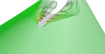
Another visualization of the datasets using stream-tubes. 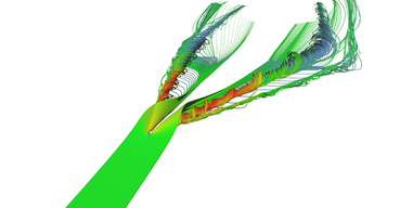
Narrow stream of air hitting the tip of the wing. 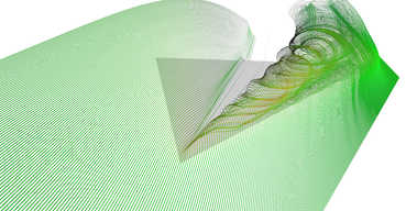
Row of stream-tubes seeded along the wing edge. 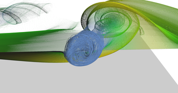
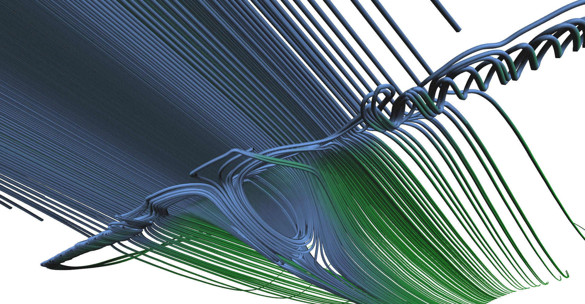
Recirculation bubble visualization. 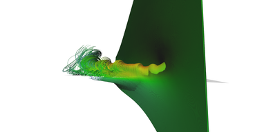
Vertical seeding of stream-tubes.
Adaptive stream lines#
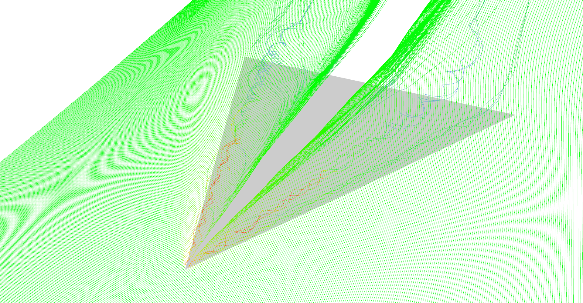
The next step towards high quality visualization is seeding the stream lines adaptively. The problem of regular seeding is that by increasing the number of lines some non-interesting areas (i.e. where flow is laminar) have too many lines but interesting areas (i.e. where flow is turbulent) could benefit from more lines.
Figure 12 shows a comparison between regular and adaptive stream lines seeding. It is nicely visible that areas with linear flow are subdivided significantly less than areas with vortices.
Regular vs. adaptive (pair 1, regular). 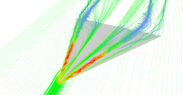
Regular vs. adaptive (pair 1, adaptive). Area near the tip of the wing is sampled much more because air is forming vortices there. 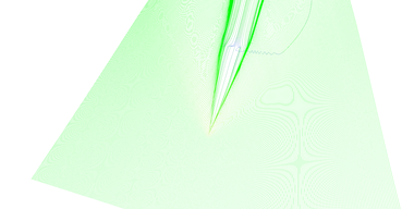
Regular vs. adaptive (pair 2, regular). 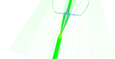
Regular vs. adaptive (pair 2, adaptive). Adaptive seeding revealed important features. 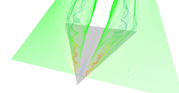
Regular vs. adaptive (pair 3, regular). 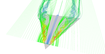
Regular vs. adaptive (pair 3, adaptive). 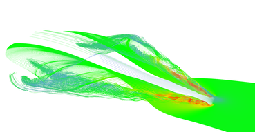
Regular vs. adaptive (pair 4, regular). 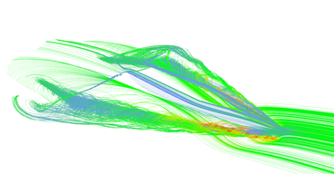
Regular vs. adaptive (pair 4, adaptive). 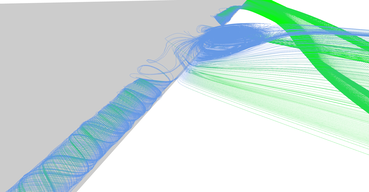
Regular vs. adaptive (pair 5, regular). 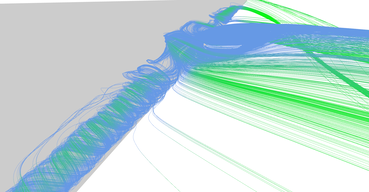
Regular vs. adaptive (pair 5, adaptive).
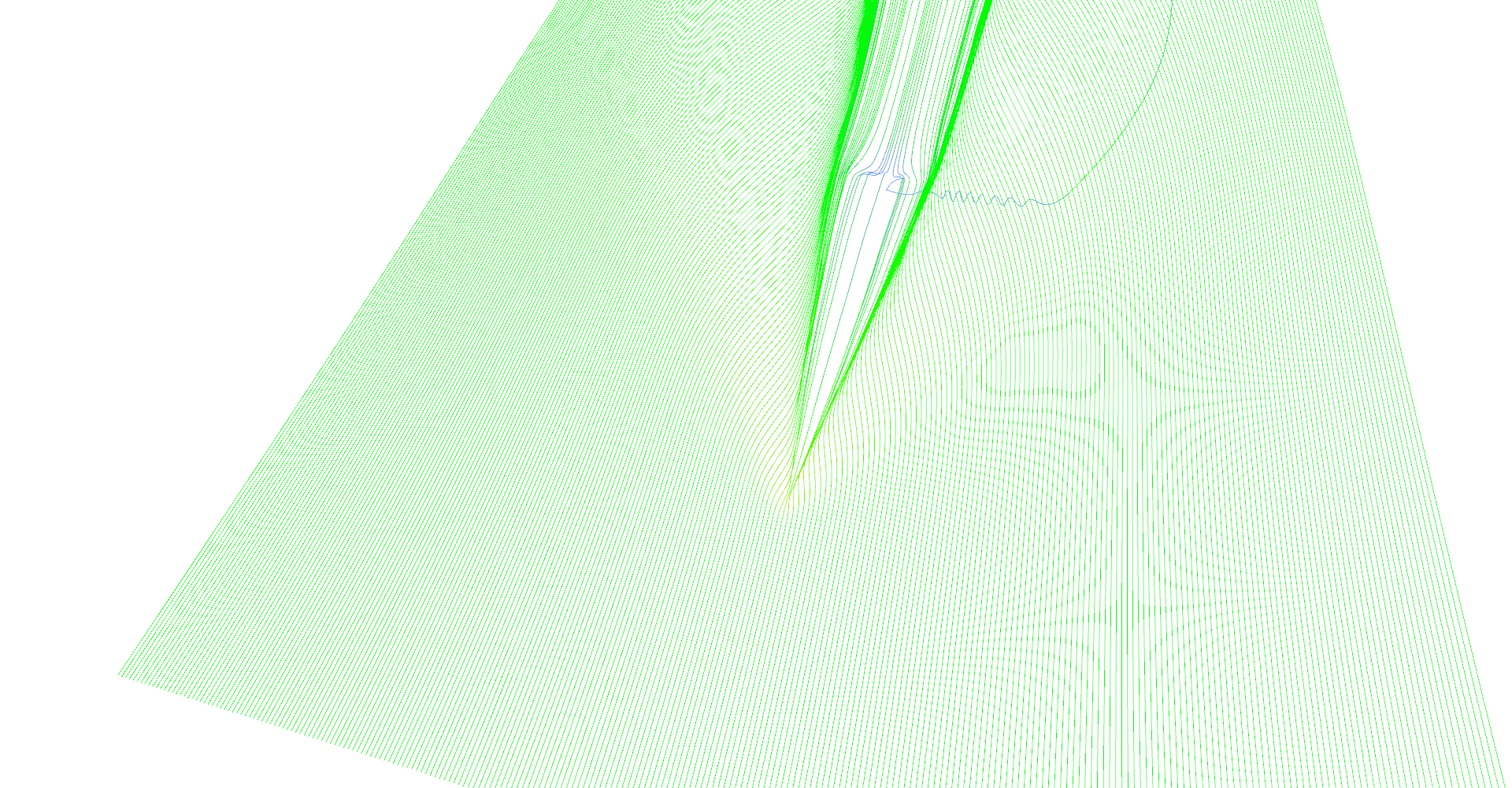
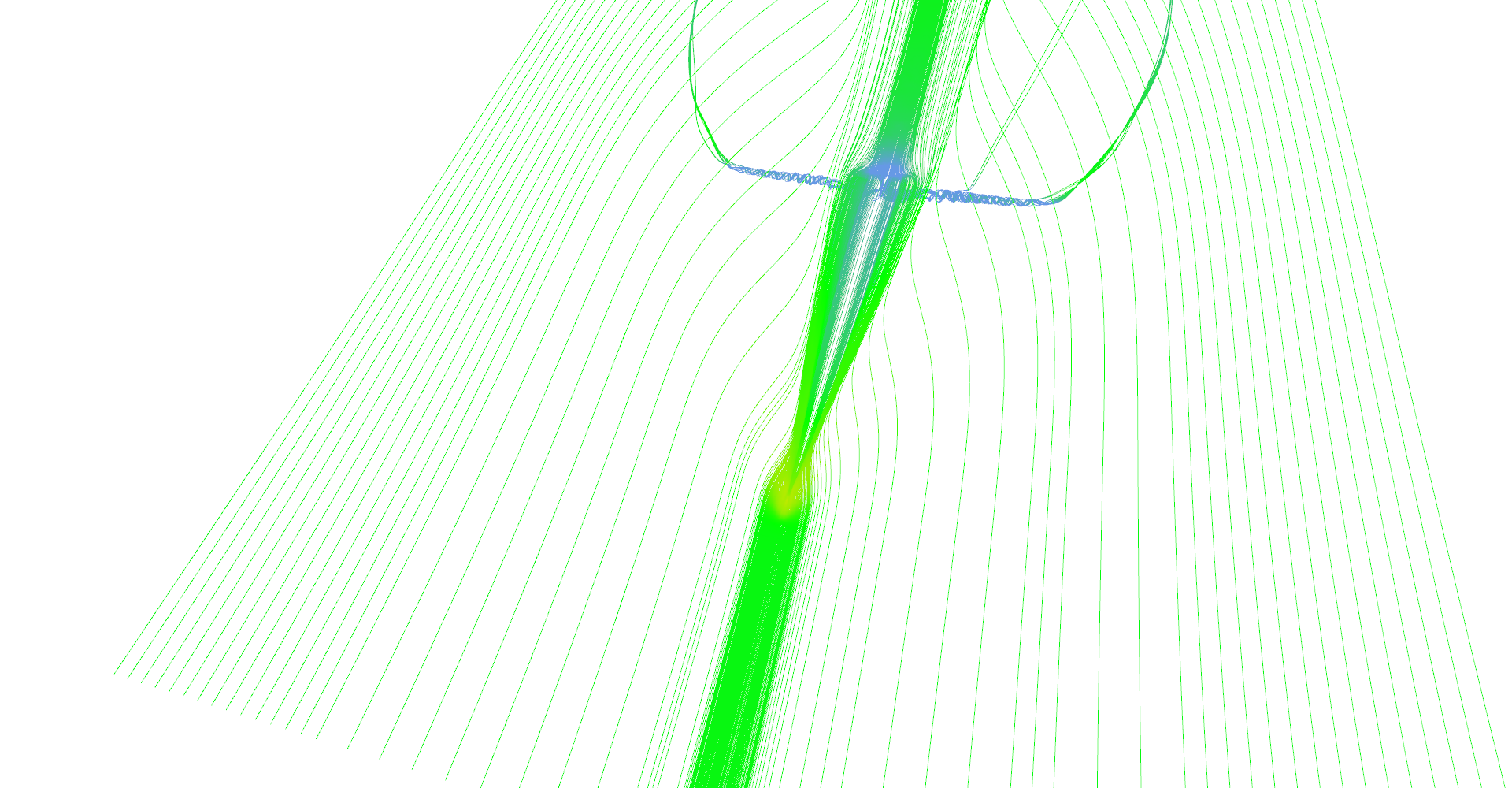
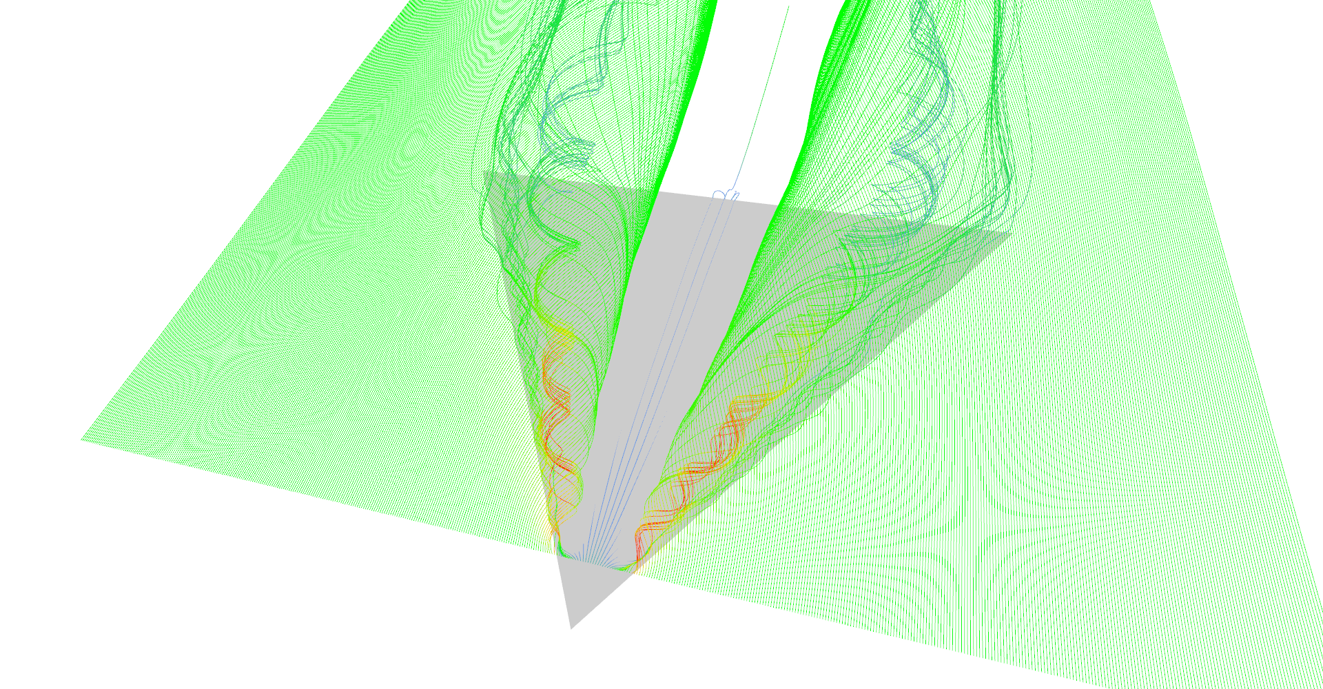
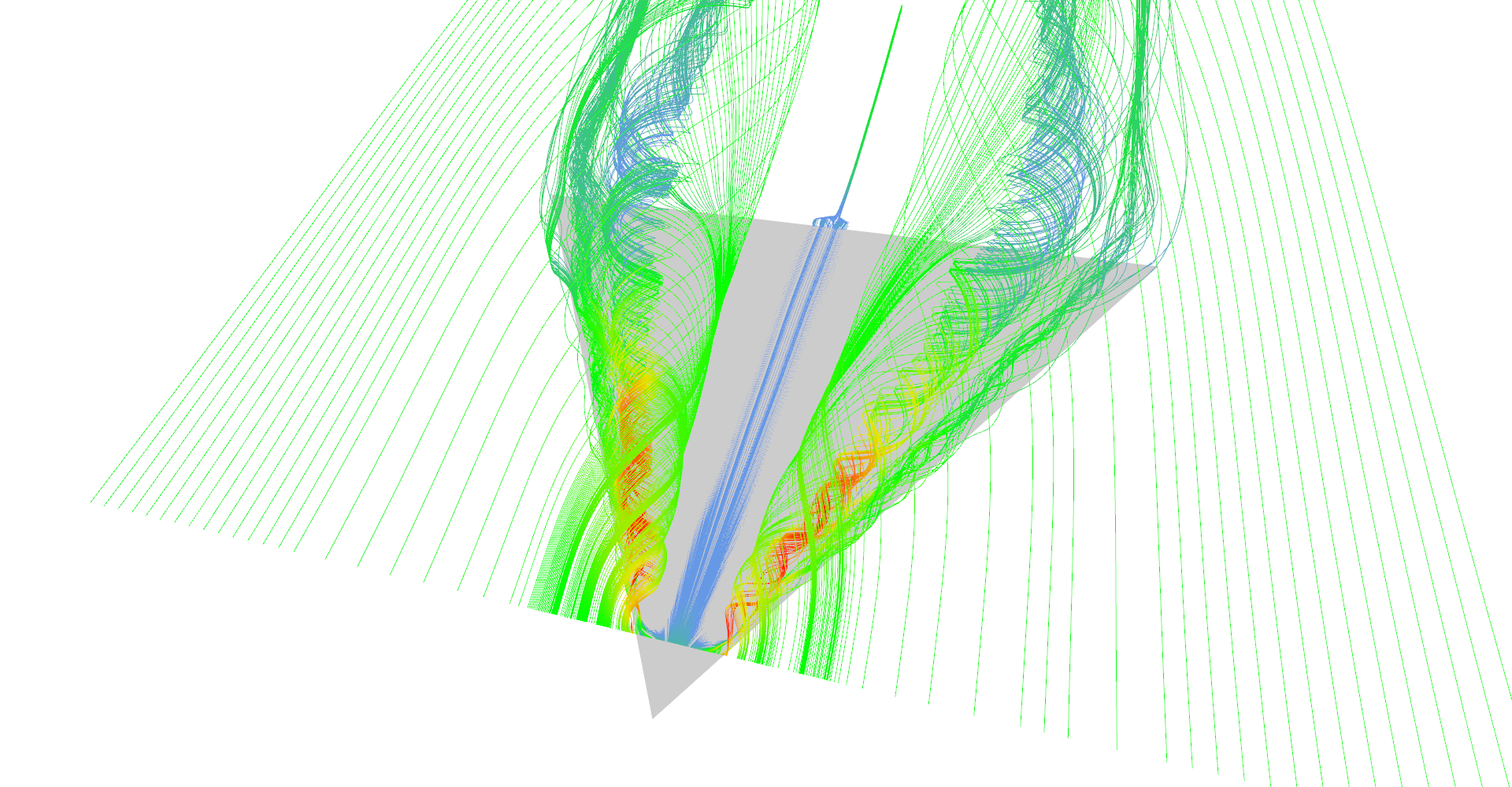
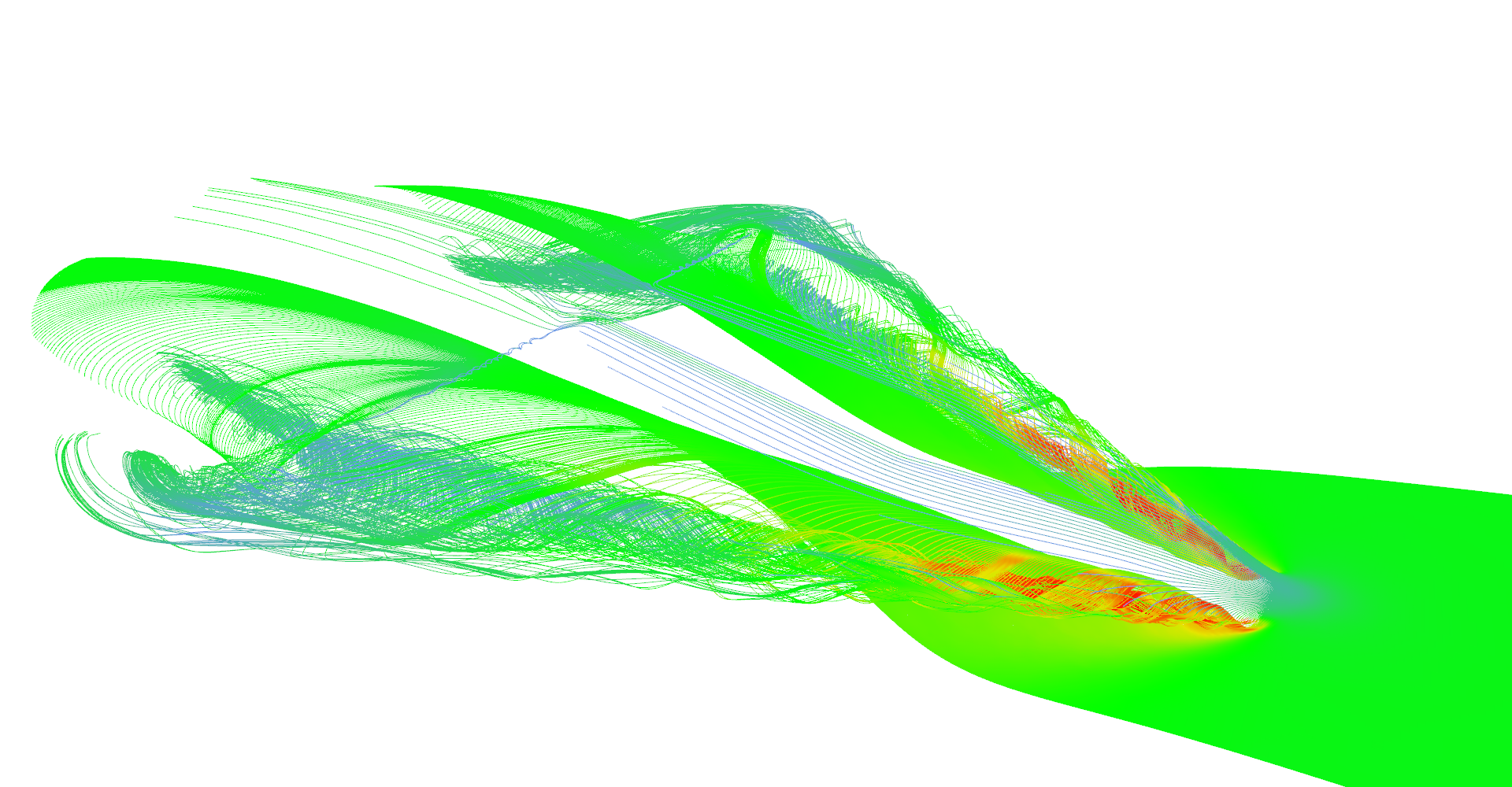
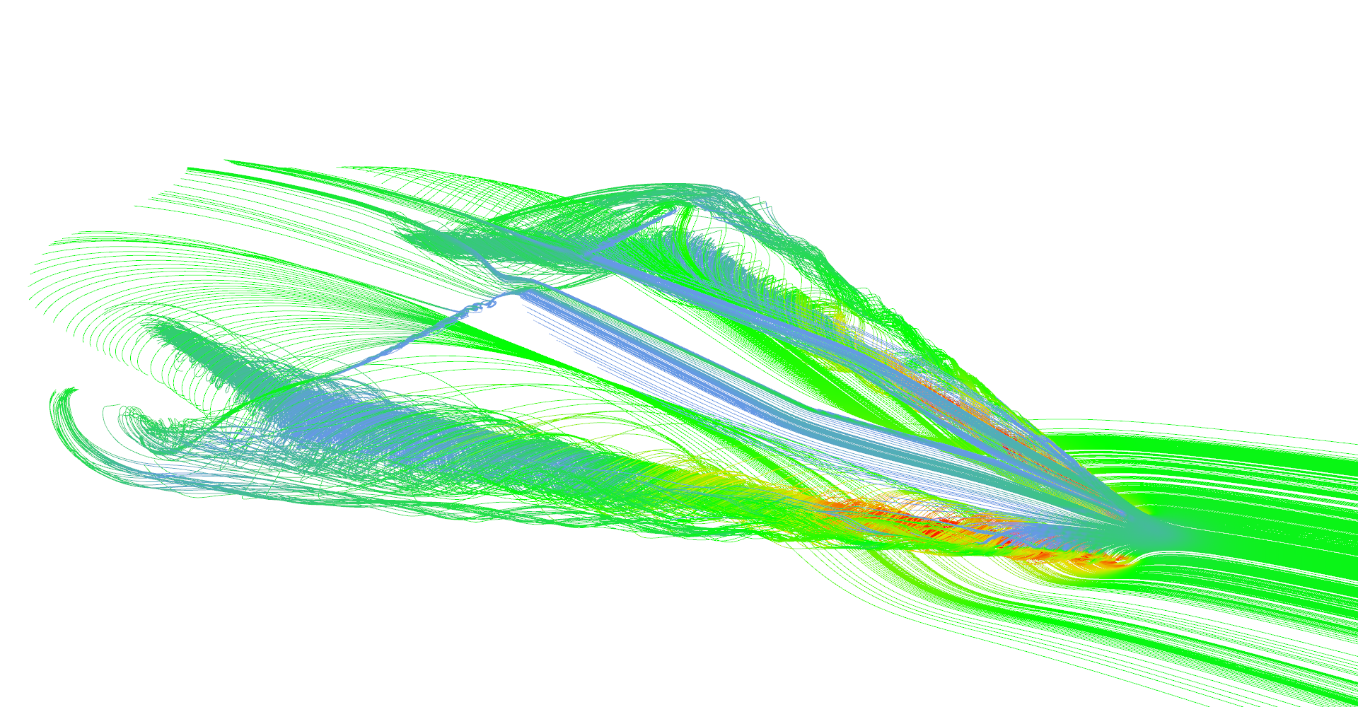
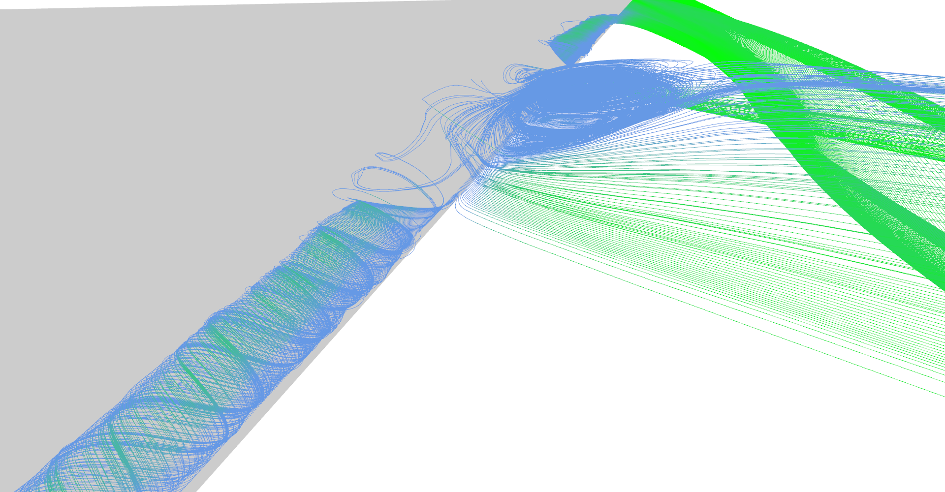
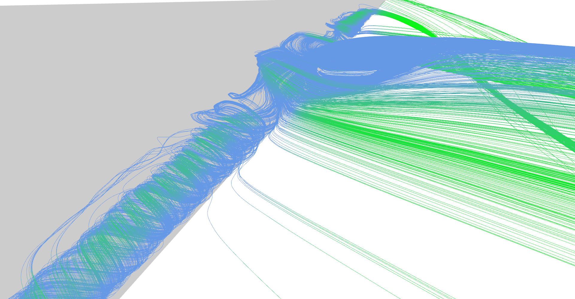
The true challenge is to implement an adaptive algorithm on GPU. It is very hard and performance costly to do thread communication on GPU. My algorithm uses two different CUDA kernels, one for control of adaptivity and the second for evaluation of stream lines themselves. Both algorithms are alternately invoked by CPU. This makes effectivity of overall algorithm worse than non-adaptive version but results are much better and overall slow-down is not very significant.
Also, memory management is not simple because you need to allocate all memory needed for GPU run before you start the kernel. Algorithm is designed in a way that space for maximum amount of lines is allocated and then adaptive algorithm is filling it till it reaches the limit.
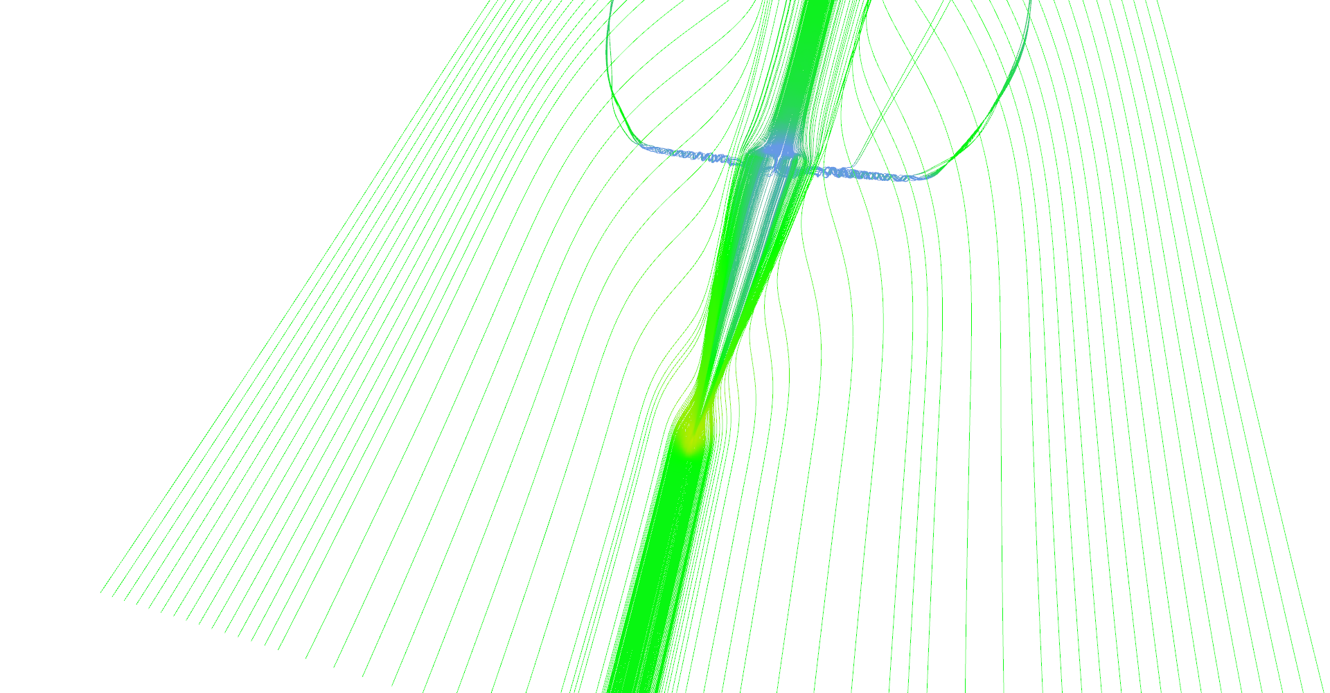
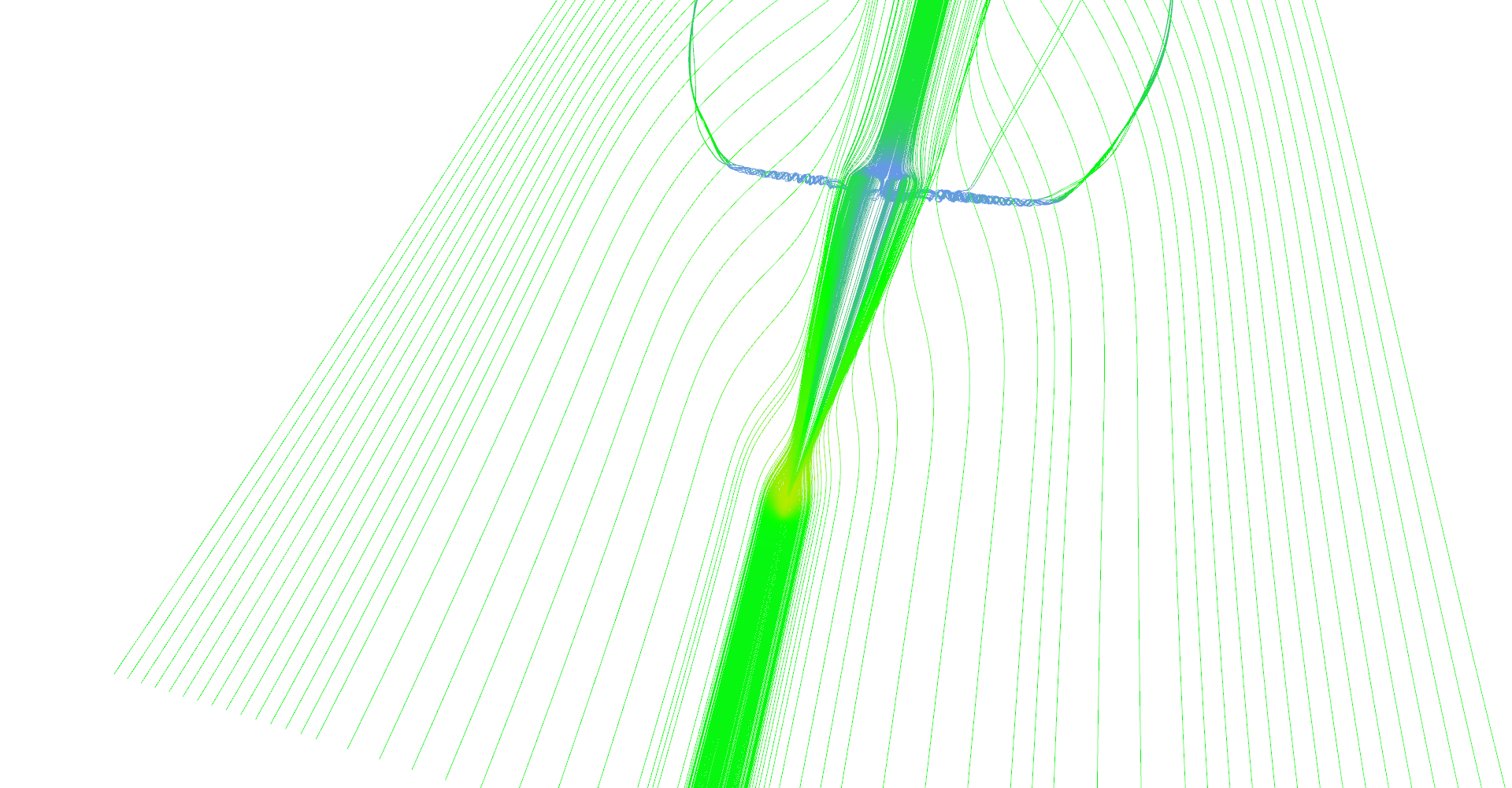
The adaptivity is implemented as subdivision. Starting with two stream lines, algorithm is adding new seeds in between stream lines which diverged (i.e. are too far from each other). Code listing 12 shows kernel for coordination of adaptivity. The input is an array of line pair indices which are neighbors and need to be considered for divergence. Divergence is determined by 32 samples among stream lines. If any of those samples is further than maximum allowed distance, a new seed is seeded in between them. Output is list of neighboring line pairs as well. Notice that clever usage of line pair indices allows subdividing lines which are at arbitrary positions in memory buffer.
This process tends to be quite slow at the beginning because the number of new lines in the n-th iteration is 2n. To speed up the start, the number of added seeds is determined based on the maximal distance between two stream lines.
1
uint newLines = (uint)sqrtf(maxDist / maxAllowedLineDist);
Another nice feature of this code is usage of atomic operations for use of a static array as a dynamic array. Because it is impossible to know in advance how many new seeds will be produced by subdivision kernel, array is allocated for maximum number of seeds and every thread tries to add one more. The variable responsible for tracking the number of elements in the array is atomically incremented and if the count is smaller than maximum allowed number of elements, new seed is added. Otherwise, variable is atomically decremented.
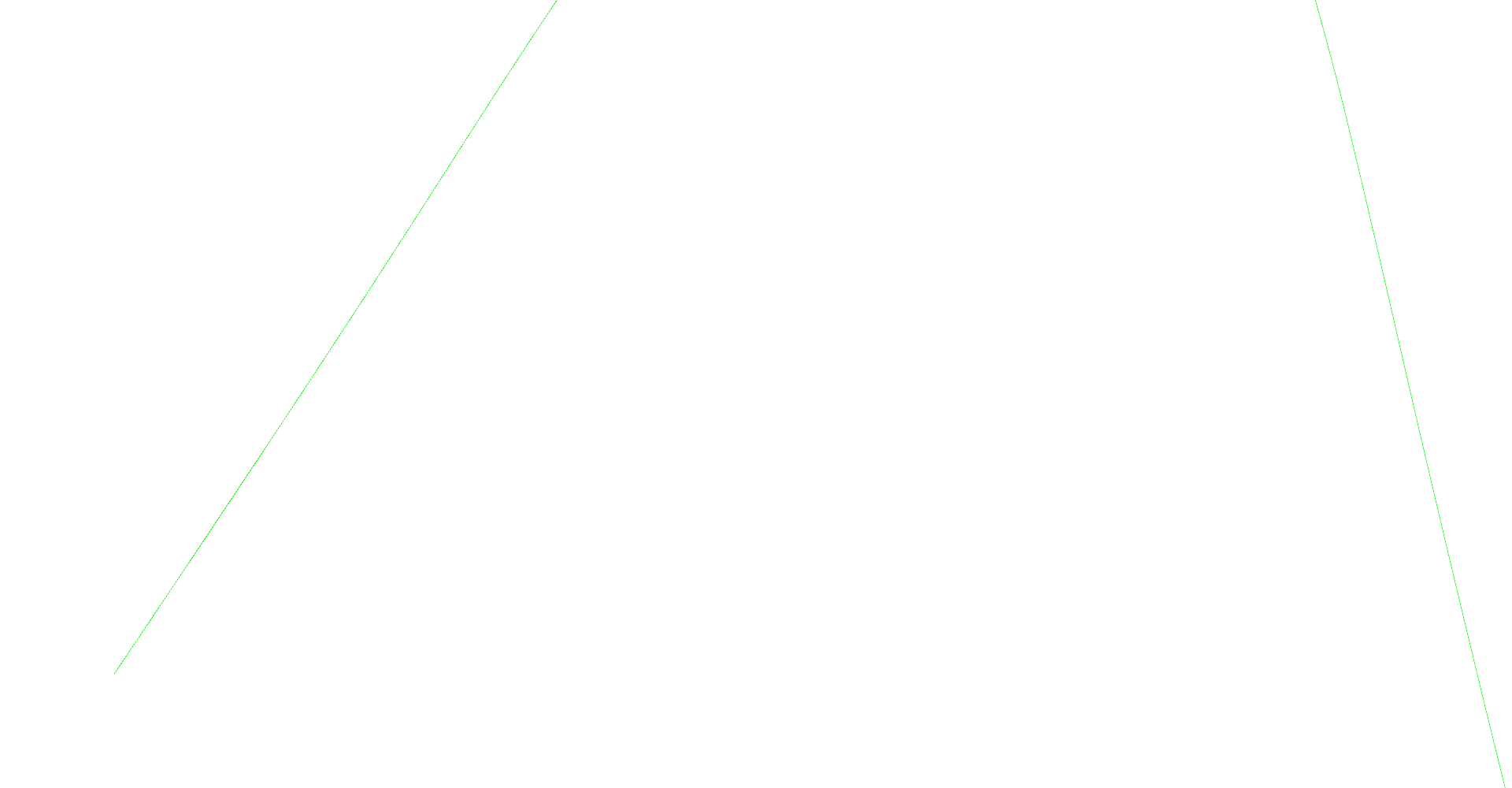
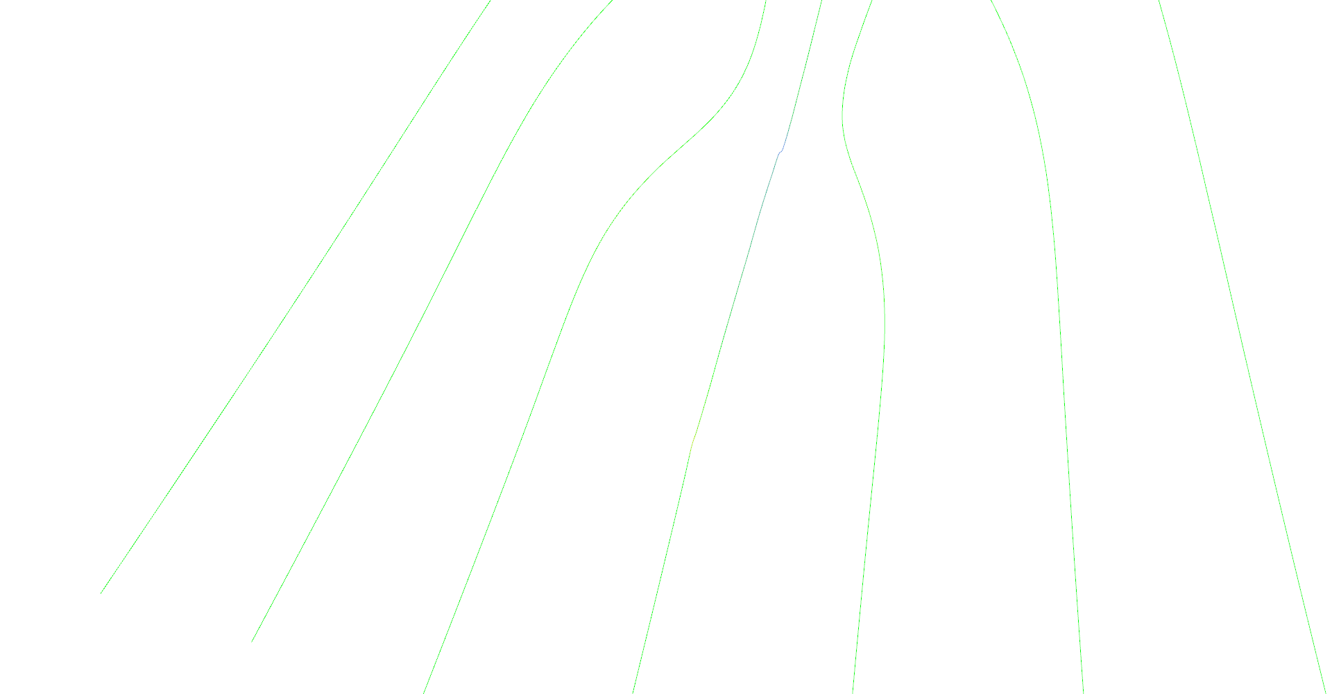
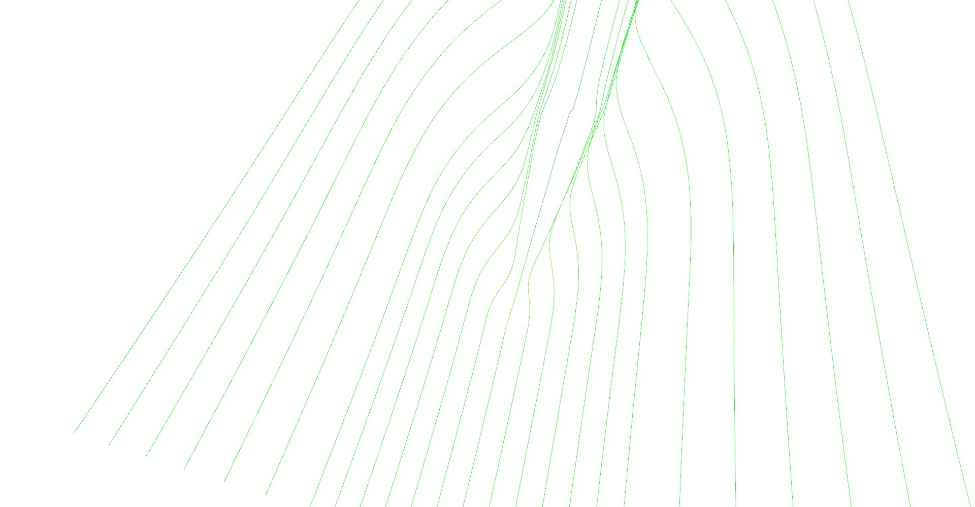
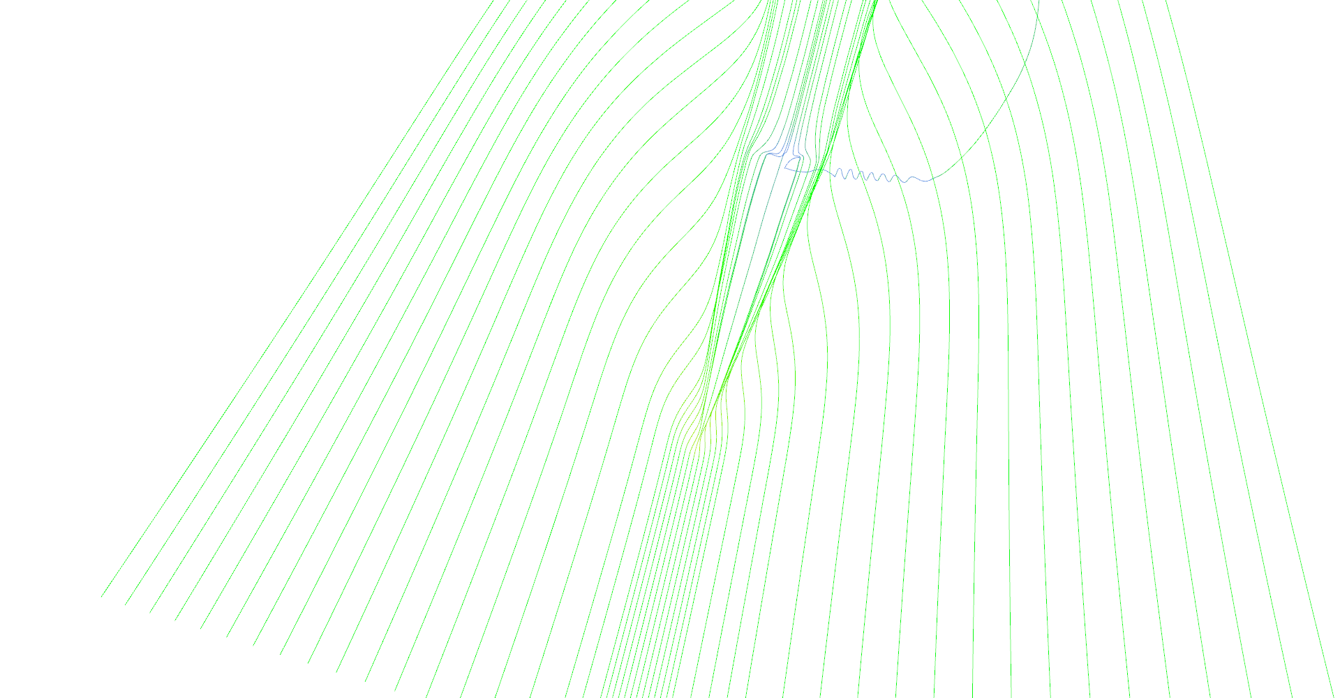
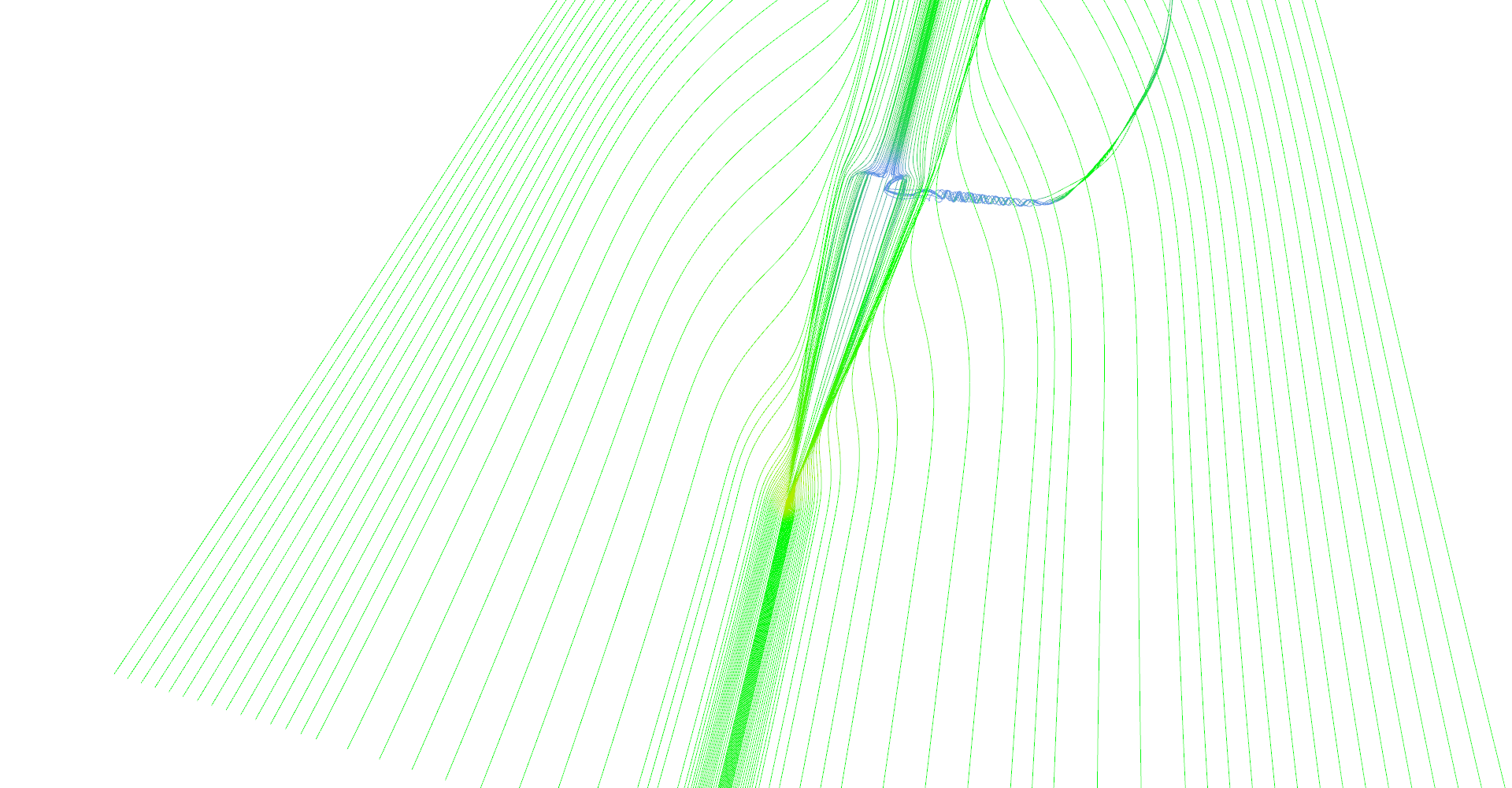
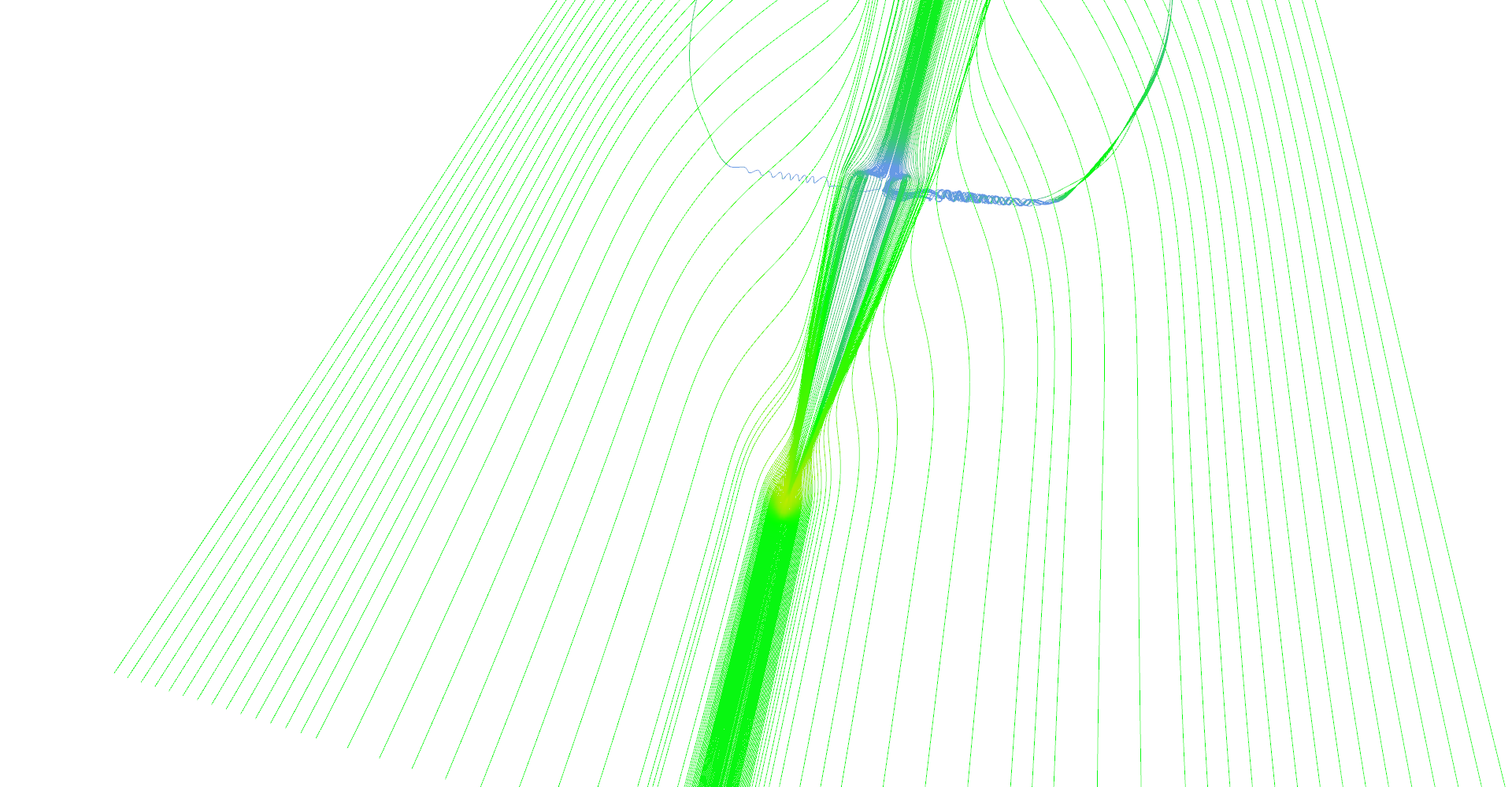
Figure 13 shows progression of adaptive stream line seeding algorithm iteration by iteration. Lines are very thin and hard to see, please click the thumbnails for a larger image.
1
2
3
4
5
6
7
8
9
10
11
12
13
14
15
16
17
18
19
20
21
22
23
24
25
26
27
28
29
30
31
32
33
34
35
36
37
38
39
40
41
42
43
44
45
46
47
48
49
50
51
52
53
54
55
56
__global__ void computeLineAdaptiveExtensionKernel(
		float maxAllowedLineDist, uint2* linePairs, uint linePairsCount,
		float3* lineVertices, uint verticesPerLine, uint verticesPerSample,
		uint* lineLengths, float3* seeds, uint2* outLinePairs,
		uint* outPairsIndex, uint* outLinesIndex, uint linesMaxCount) {

	uint id = __umul24(blockIdx.x, blockDim.x) + threadIdx.x;
	if (id >= linePairsCount) {
		return;
	}

	uint2 currPair = linePairs[id];
	uint outPairIndex = atomicAdd(outPairsIndex, 1);
	// Preserve original pair.
	outLinePairs[outPairIndex].x = currPair.x;
	outLinePairs[outPairIndex].y = currPair.y;

	uint count = min(lineLengths[currPair.x], lineLengths[currPair.y]);
	if (count < 2) {
		return;  // One of lines too short.
	}

	// Test 32 samples for divergence.
	float maxDist = 0;
	for (uint i = 0; i < count; i += count / 32) {
		float3 v1 = lineVertices[currPair.x * verticesPerLine + i * verticesPerSample];
		float3 v2 = lineVertices[currPair.y * verticesPerLine + i * verticesPerSample];
		maxDist = max(maxDist, length(v1 - v2));
	}

	if (maxDist < maxAllowedLineDist) {
		return;  // Lines do not diverged.
	}

	uint newLines = (uint)sqrtf(maxDist / maxAllowedLineDist);

	uint outLineIndex = atomicAdd(outLinesIndex, newLines);
	if ((outLineIndex + newLines) >= linesMaxCount) {
		atomicAdd(outLinesIndex, -newLines);
		return;  // Not enough space for new seeds.
	}

	float3 seedStep = (seeds[currPair.y] - seeds[currPair.x]) / (newLines + 1);

	uint lastOutPairIndex = outPairIndex;
	for (uint i = 0; i < newLines; ++i) {
		seeds[outLineIndex + i] = seeds[currPair.x] + (i + 1) * seedStep;
		// Insert new pair (like in linked-list).
		uint outPairIndex = atomicAdd(outPairsIndex, 1);
		outLinePairs[lastOutPairIndex].y = outLineIndex + i;
		outLinePairs[outPairIndex].x = outLineIndex + i;
		outLinePairs[outPairIndex].y = currPair.y;

		lastOutPairIndex = outPairIndex;
	}
}
Step 1 of adaptive seeding algorithm. 
Step 2 of adaptive seeding algorithm. 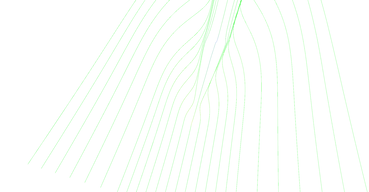
Step 3 of adaptive seeding algorithm. 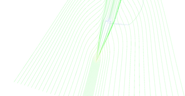
Step 4 of adaptive seeding algorithm. 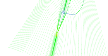
Step 5 of adaptive seeding algorithm. 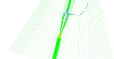
Step 6 of adaptive seeding algorithm. 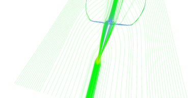
Step 7 of adaptive seeding algorithm. 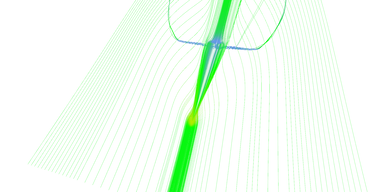
Step 8 of adaptive seeding algorithm.
5. Visualization using stream surfaces#
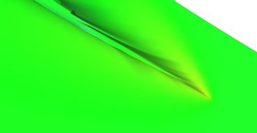
The last visualization technique is stream surfaces. The idea is very simple: seed stream lines on some curve (e.g. line) and triangulate space between each neighboring pair to create a surface. The advantage of stream surfaces is the fact that they can be shaded thus, easily seen in 3D.
The problem is that some lines that started very close to each other diverge later in the vector field. The triangulation needs to stop if lines diverge, otherwise visualization will be full of overlapping triangles. Figure 14 shows an image sequence of a stream surface seeded along a line which is moving from front to back of the delta wing.
Triangulation of stream lines to form stream surface is done by pairs, every pair on a separate CUDA thread. Triangulation of single pair of lines is implemented in following fashion. Going from the first vertices of the lines, there are always two ways to add the next triangle:
- Create a triangle from indices
iandi + 1from the first line and indexjfrom second line, - or take index
ifrom the first and indicesjandj + 1from the second line.
The one which is "better" is picked and this continues till all points are triangulated or lines are too far away. The better triangle is determined as the triangle with the shorter edge between stream lines. Code listing 13 shows simplified CUDA kernel for creation of stream surface from stream line pairs (many implementation details omitted).
1
2
3
4
5
6
7
8
9
10
11
12
13
14
15
16
17
18
19
20
21
22
23
24
25
26
27
28
29
30
31
32
33
34
35
36
37
38
39
40
41
42
43
44
45
46
47
48
49
50
51
52
53
54
55
56
57
58
59
60
61
62
63
64
65
66
67
68
69
__global__ void computeStreamSurfaceKernel(uint2* linePairs,
		uint linePairsCount, float3* lineVertices,
		uint verticesPerLine, uint* lineLengths,
		uint3* outFaces, uint* outFacesCounts, float3* outNormals) {

	uint id = __umul24(blockIdx.x, blockDim.x) + threadIdx.x;
	if (id >= linePairsCount) {
		return;
	}

	uint2 currPair = linePairs[id];
	uint2 lengths = make_uint2(lineLengths[currPair.x], lineLengths[currPair.y]);

	if (lengths.x < 2 || lengths.y < 2) {
		outFacesCounts[id] = 0;
		return;  // Lines too short for triangulation.
	}

	uint line1Offset = currPair.x * verticesPerLine;
	uint line2Offset = currPair.y * verticesPerLine;
	float3* line1 = lineVertices + line1Offset;
	float3* line2 = lineVertices + line2Offset;
	float3* normals1 = outNormals + line1Offset;
	float3* normals2 = outNormals + line2Offset;

	uint maxFaces = verticesPerLine * 2 - 2;
	uint3* faces = outFaces + id * maxFaces;
	uint2 currIndex = make_uint2(0, 0);

	uint faceId;
	for (faceId = 0; faceId < maxFaces; ++faceId) {
		if (currIndex.x + 1 >= lengths.x || currIndex.y + 1 >= lengths.y) {
			break;  // Reached the end of stream line.
		}

		float dist1 = (currIndex.x + 1 < lengths.x)
			? length(line1[currIndex.x + 1] - line2[currIndex.y])
			: (1.0f / 0.0f);  // Infinity.
		float dist2 = (currIndex.y + 1 < lengths.y)
			? length(line1[currIndex.x] - line2[currIndex.y + 1])
			: (1.0f / 0.0f);  // Infinity.

		uint newVertexIndex;
		float3 newVertex;
		uint2 nextIndex;

		if (dist1 <= dist2) {
			newVertexIndex = line1Offset + currIndex.x + 1;
			newVertex = line1[currIndex.x + 1];
			nextIndex = make_uint2(currIndex.x + 1, currIndex.y);
		}
		else if (dist2 < dist1) {
			newVertexIndex = line2Offset + currIndex.y + 1;
			newVertex = line2[currIndex.y + 1];
			nextIndex = make_uint2(currIndex.x, currIndex.y + 1);
		}

		faces[faceId] = make_uint3(line1Offset + currIndex.x,
			line2Offset + currIndex.y, newVertexIndex);
		float3 normal = cross(line1[currIndex.x] - line2[currIndex.y],
			newVertex - line2[currIndex.y]);
		normal = normalize(normal);
		normals1[currIndex.x] = normal;
		normals2[currIndex.y] = normal;
		currIndex = nextIndex;
	}

	outFacesCounts[id] = faceId;
}
Stream surface (1) 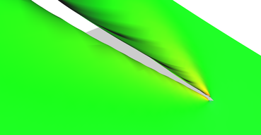
Stream surface (2) 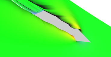
Stream surface (3) 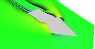
Stream surface (4) 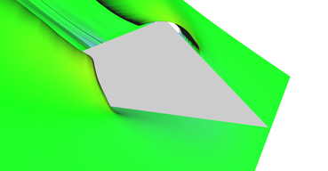
Stream surface (5) 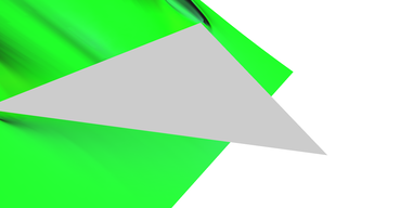
Stream surface (6)
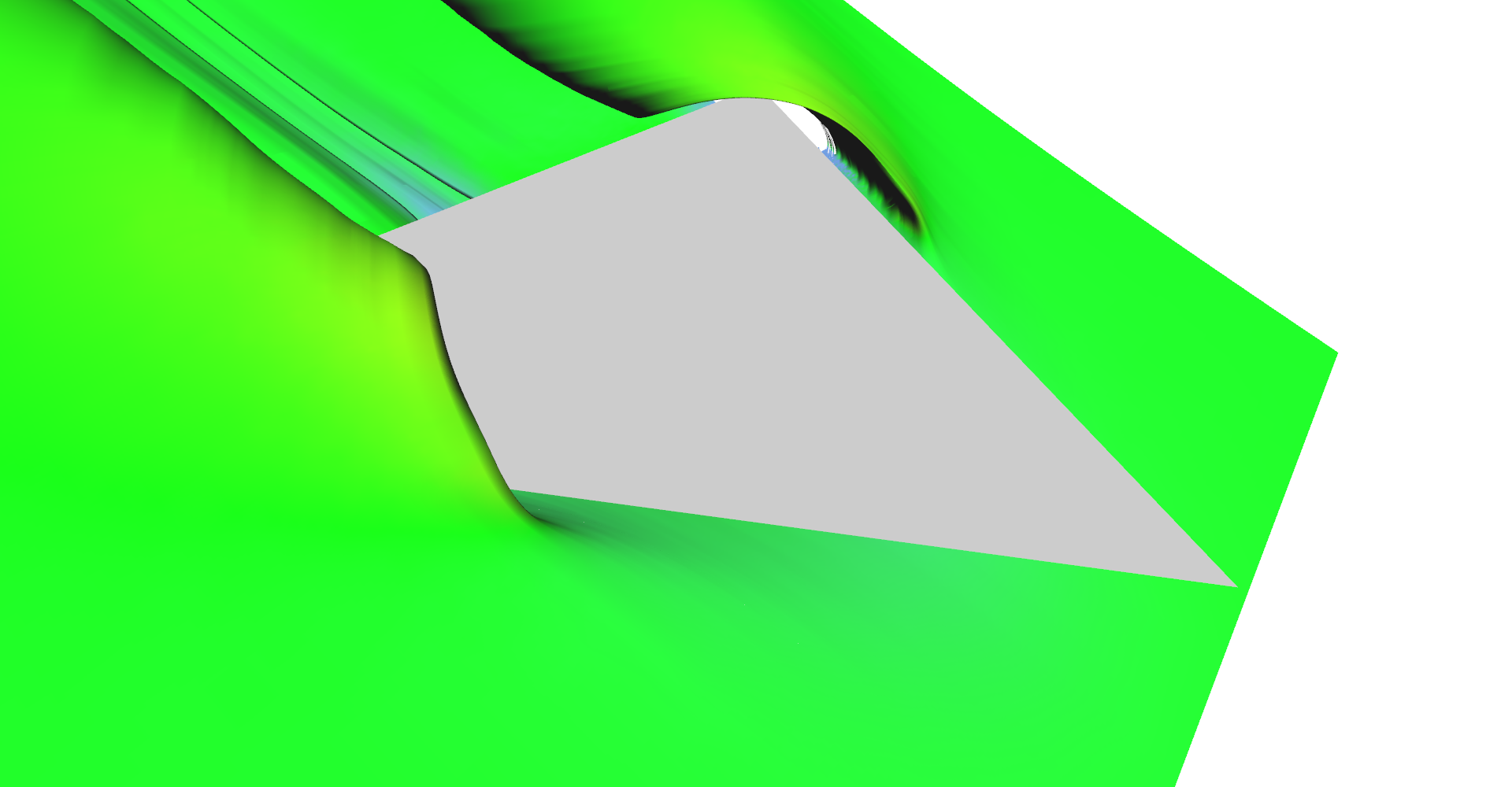
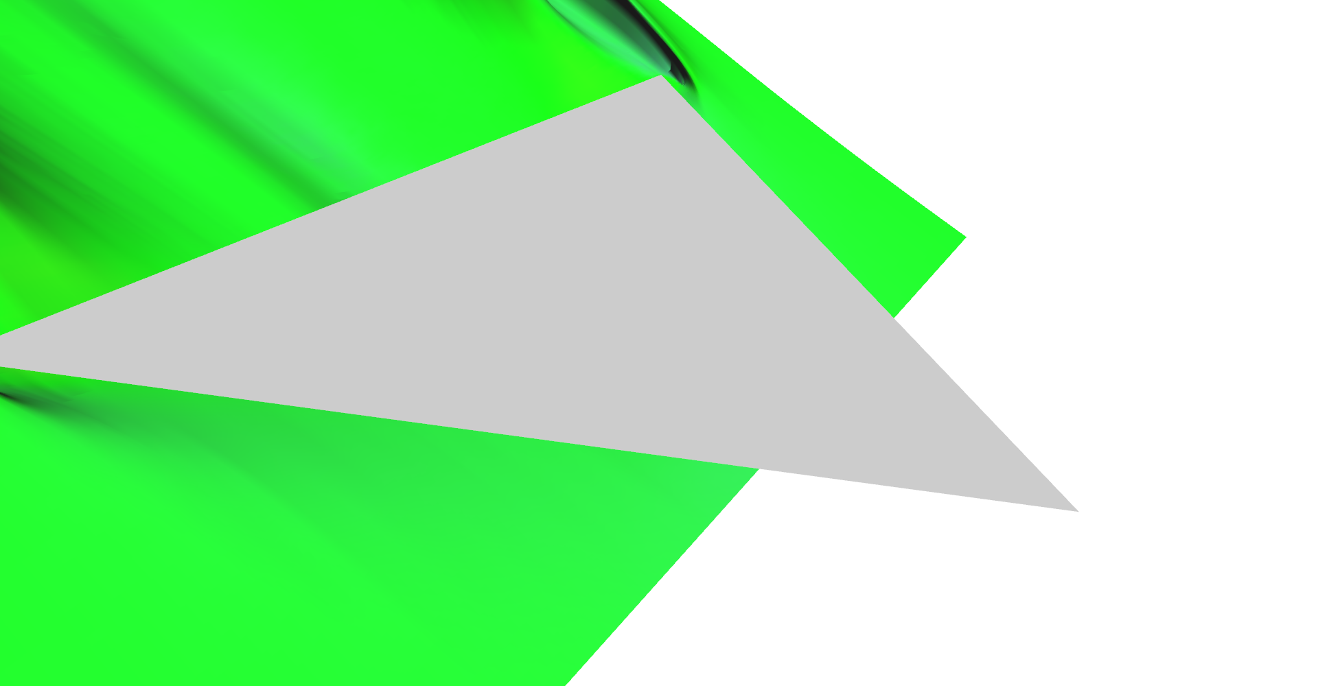
Adaptive stream surfaces#
The code for adaptive stream line seeding and code for stream surfaces generation have one important thing in common. Both algorithms work with line pairs. This means that they can be plugged together very easily (and that was the intention from the beginning).
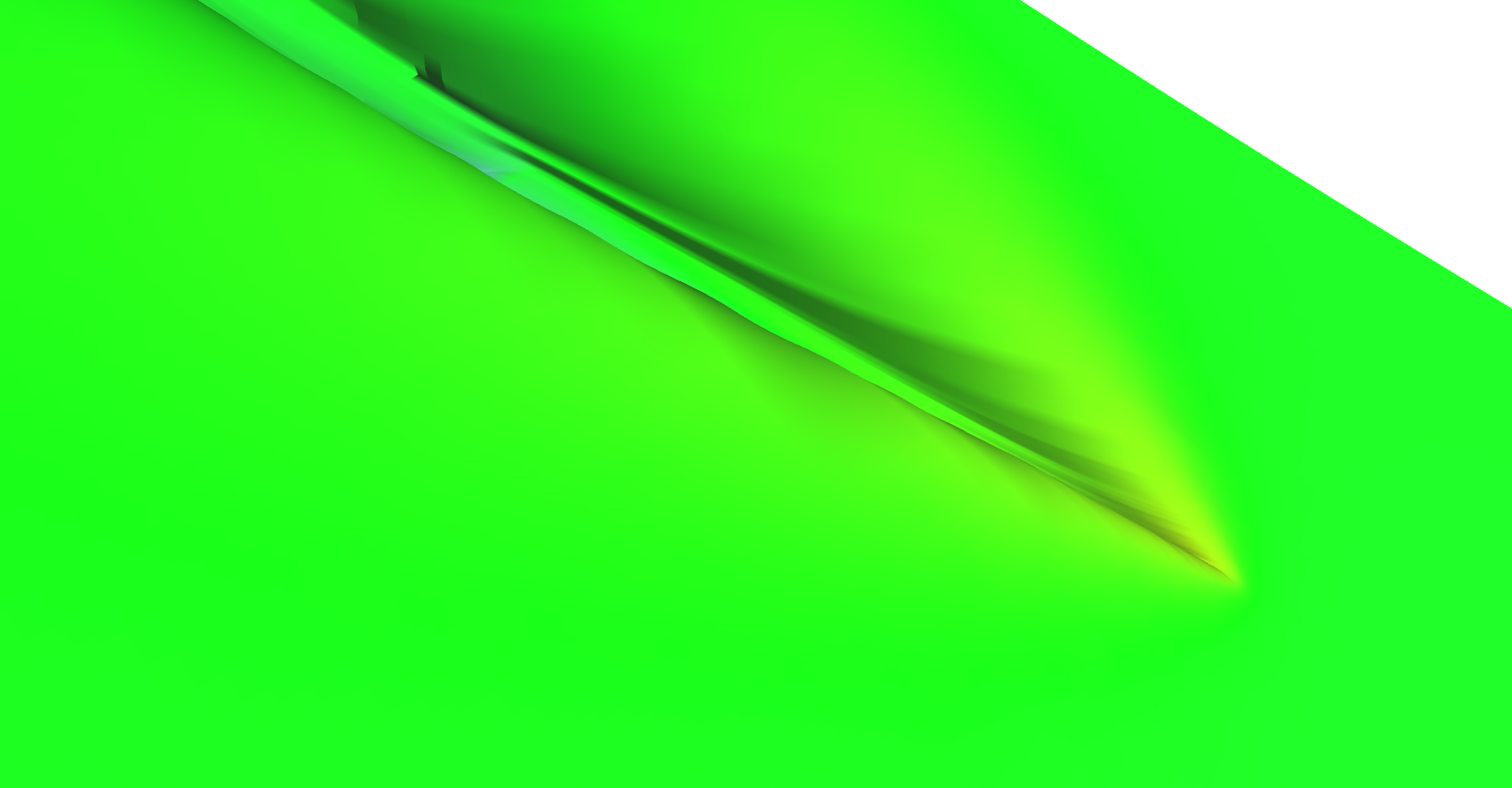
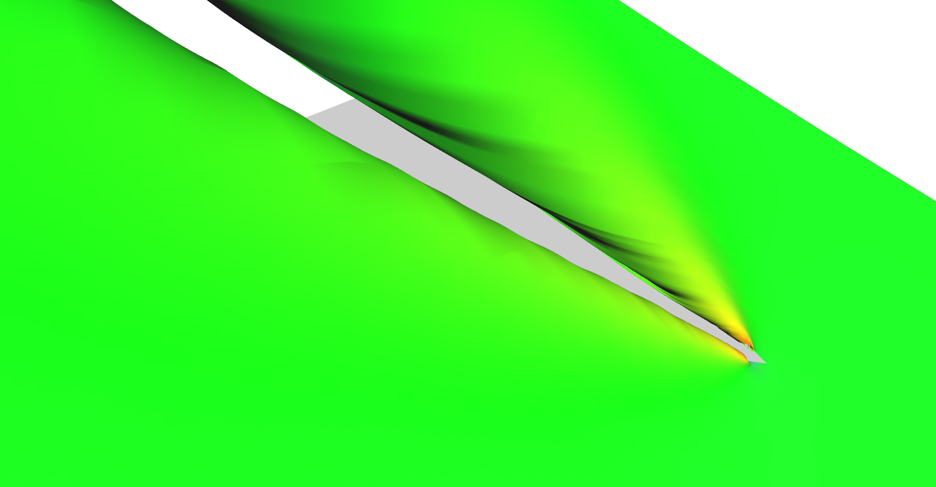
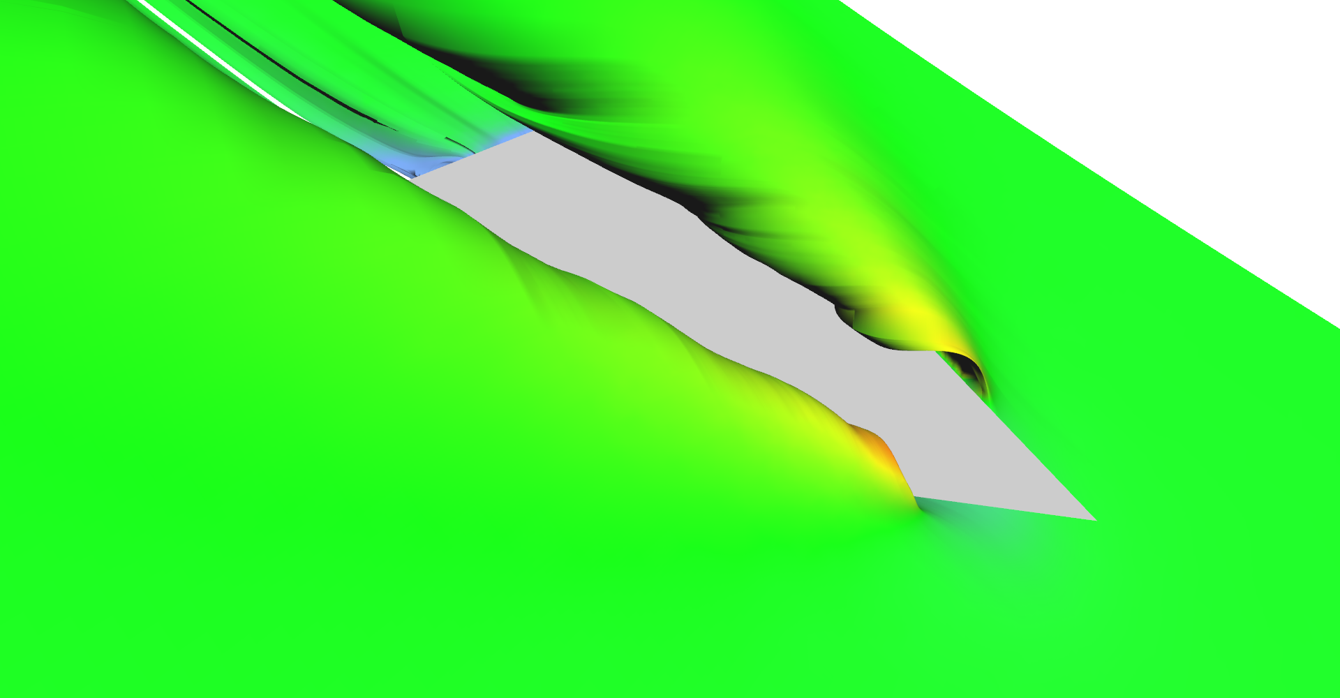
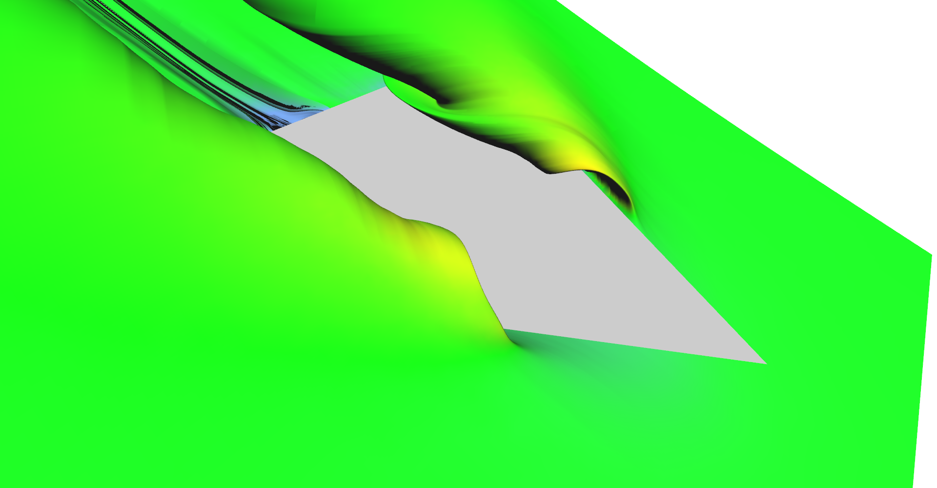
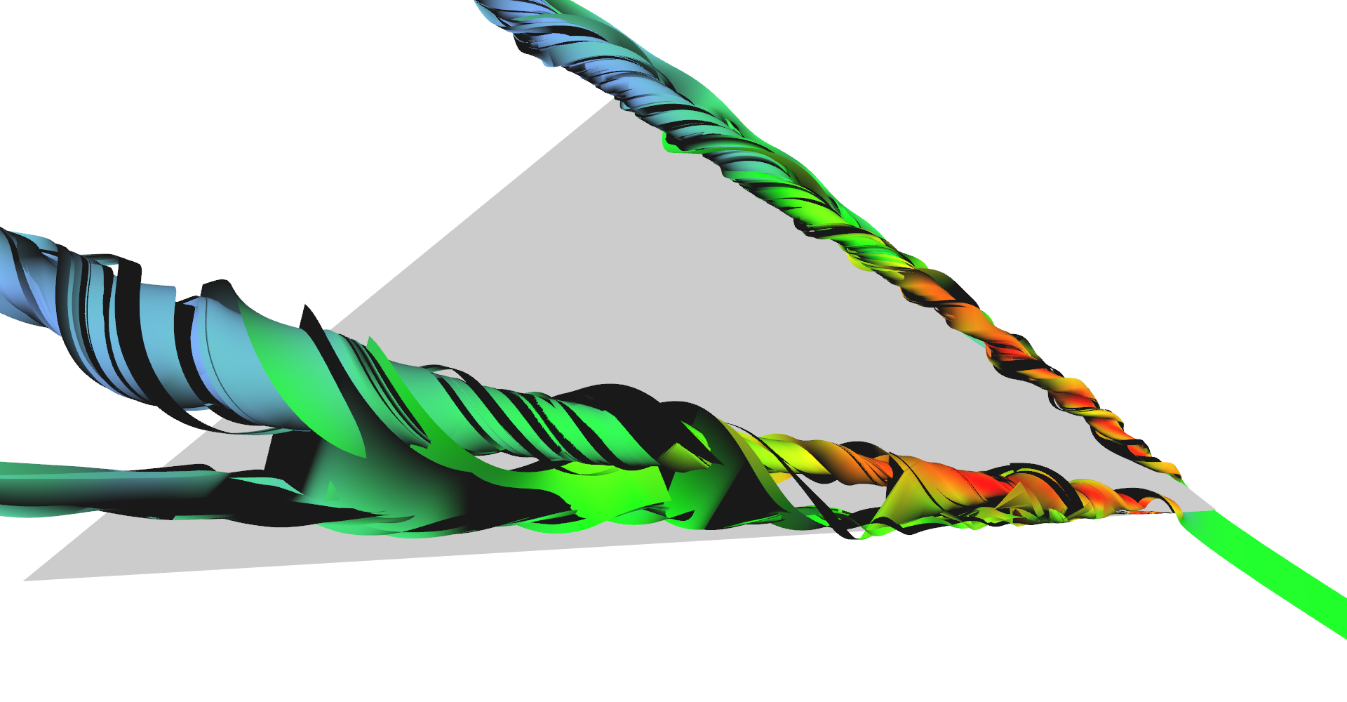
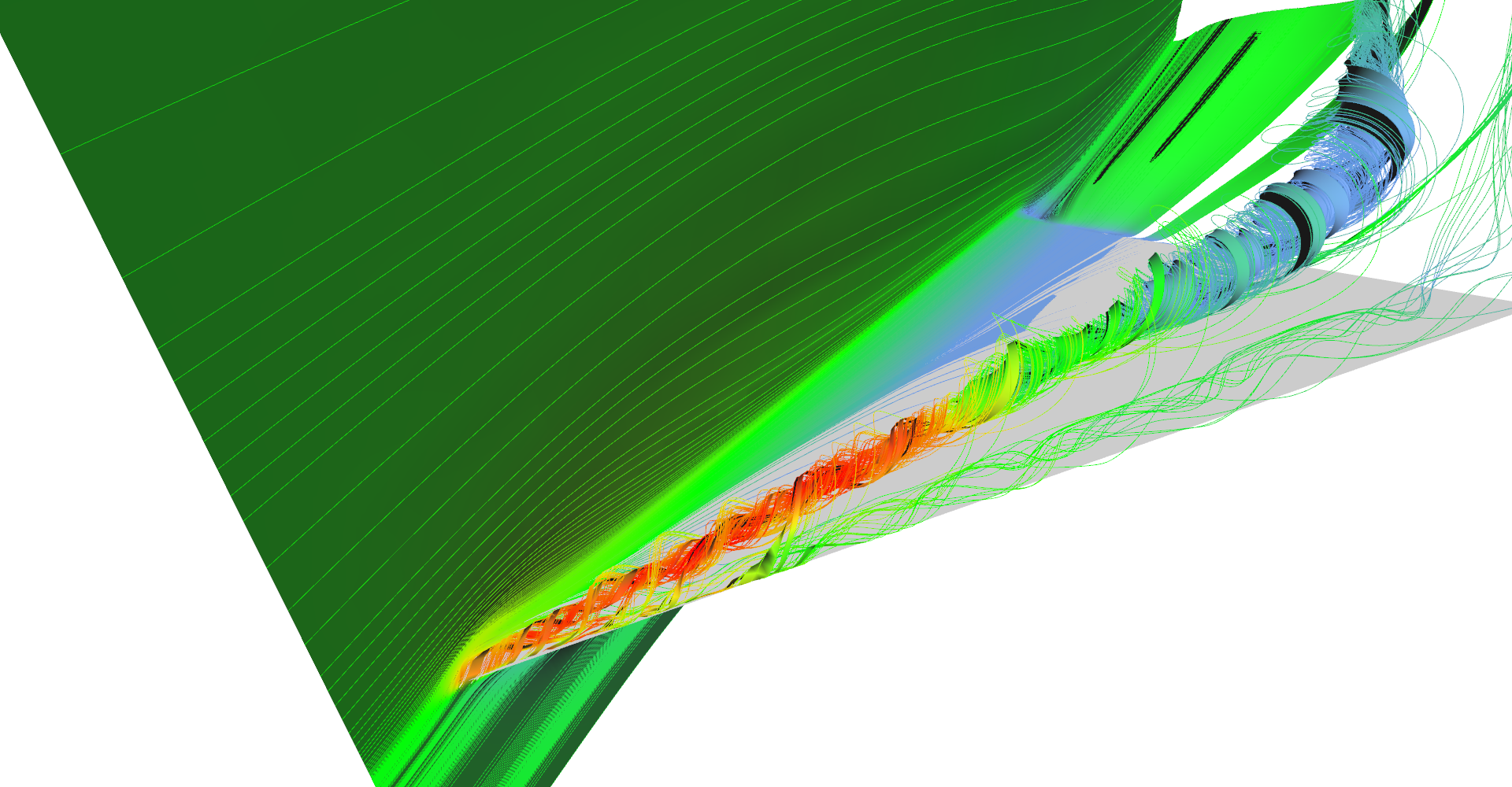
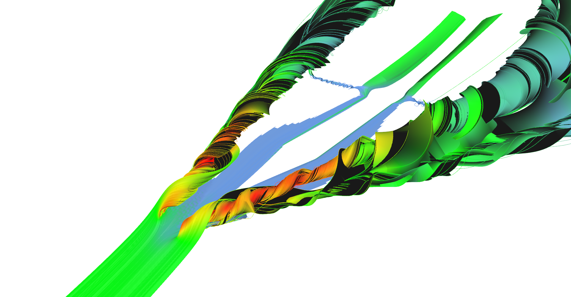
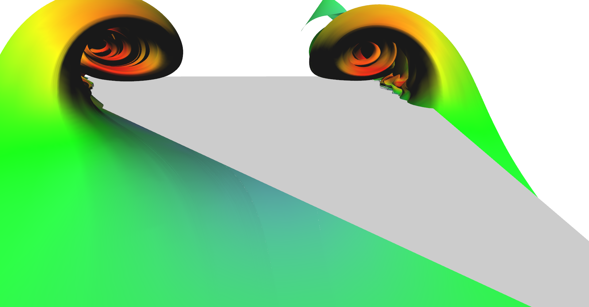
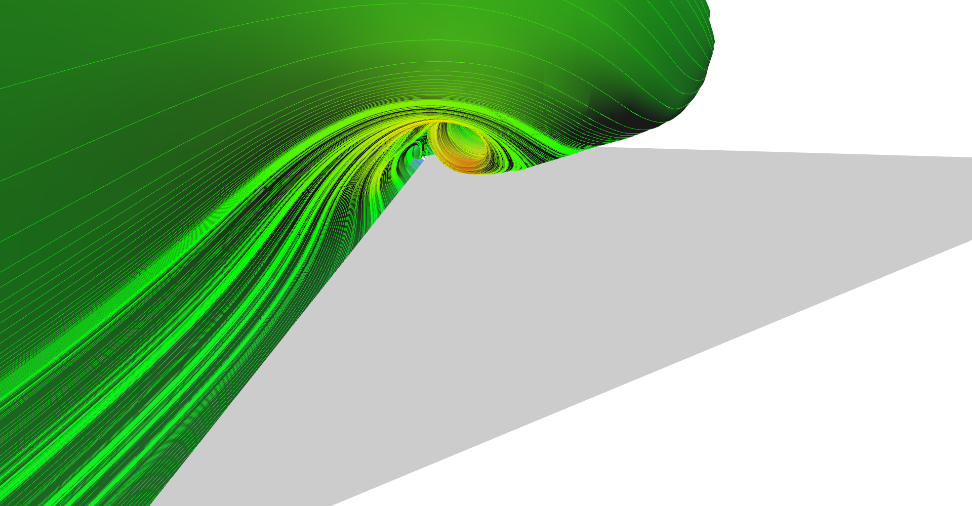
The only problem is that when line seeding is adaptive, criteria for breaking triangulation of lines which are too far away need to be adaptive as well. Triangulation needs to work properly for lines which are close to each other as well as for lines starting further apart. The solution is that the threshold for breaking is slowly adapting to the actual distance so if lines are diverging slowly, they will remain attached. This can be nicely observed at Figure 15 which shows wireframe of detail of stream surface.
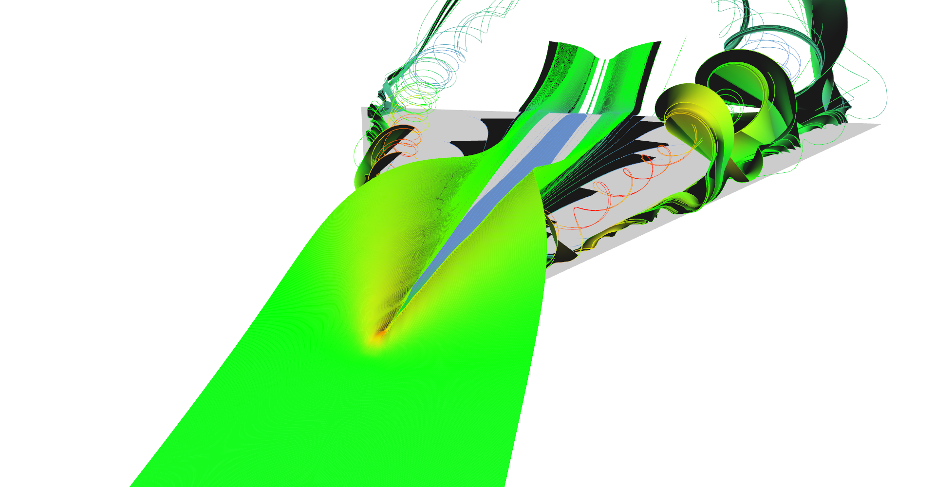
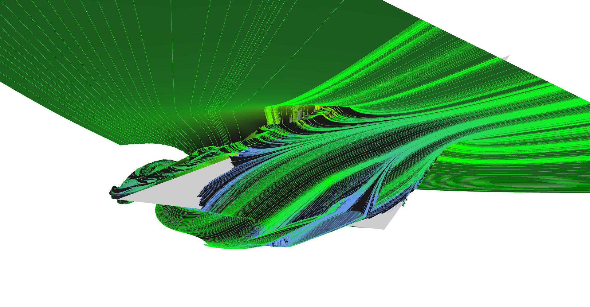
Figure 16 shows results of adaptive stream surface seeding. Some images have stream lines included in visualization too. Please note that I was not able to enable two-sided lighting model together with color material so one side of the surface is completely black.
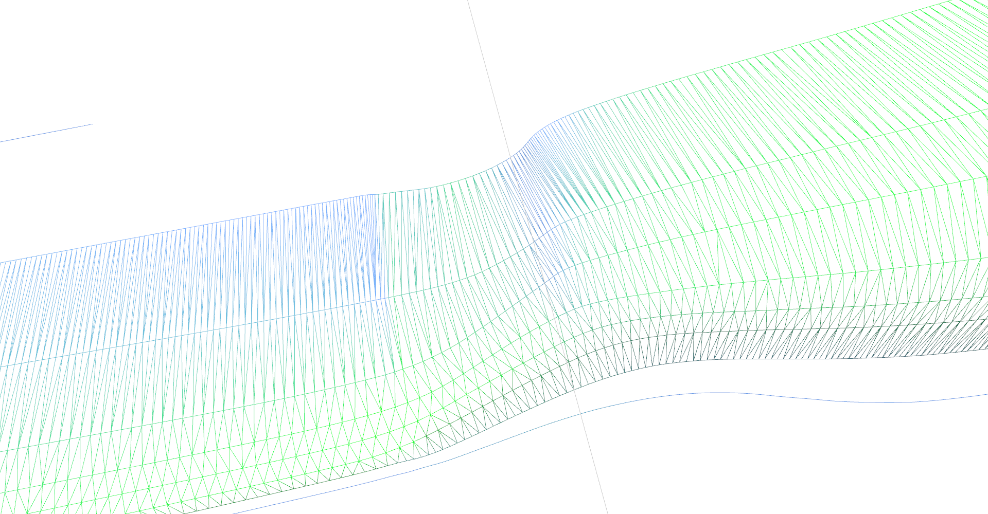 Figure 15: Adaptive triangulation detail.
Adaptive stream surface (1) 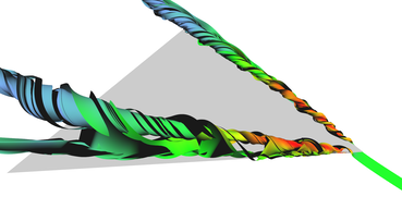
Adaptive stream surface (2) 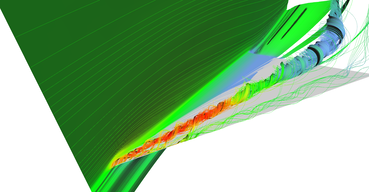
Adaptive stream surface (3) 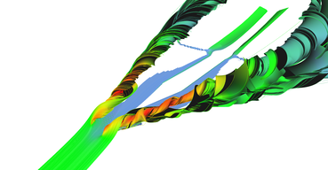
Adaptive stream surface (4) 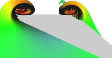
Adaptive stream surface (5) 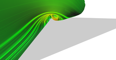
Adaptive stream surface (6)
Regular vs. adaptive seeding#
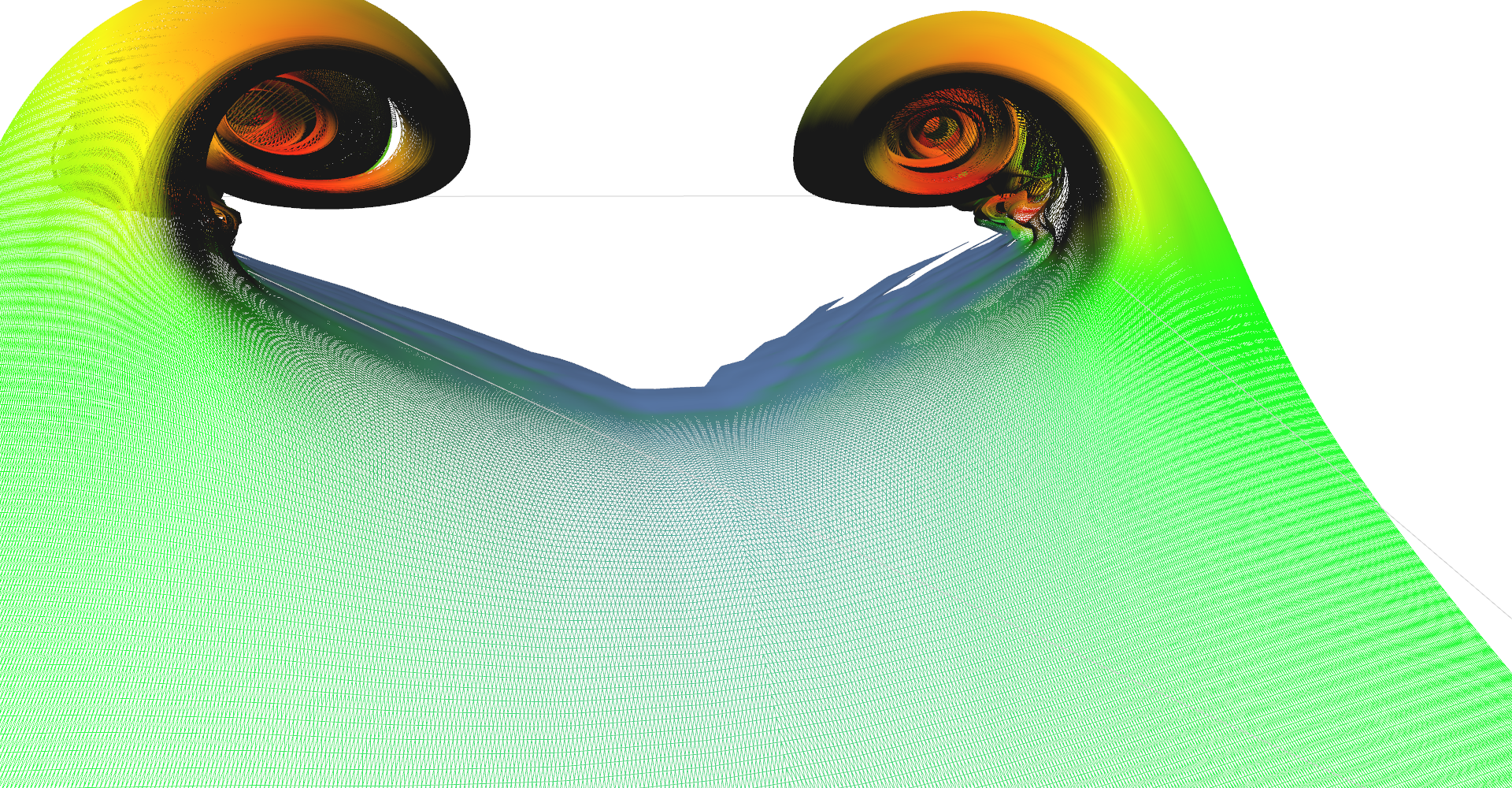
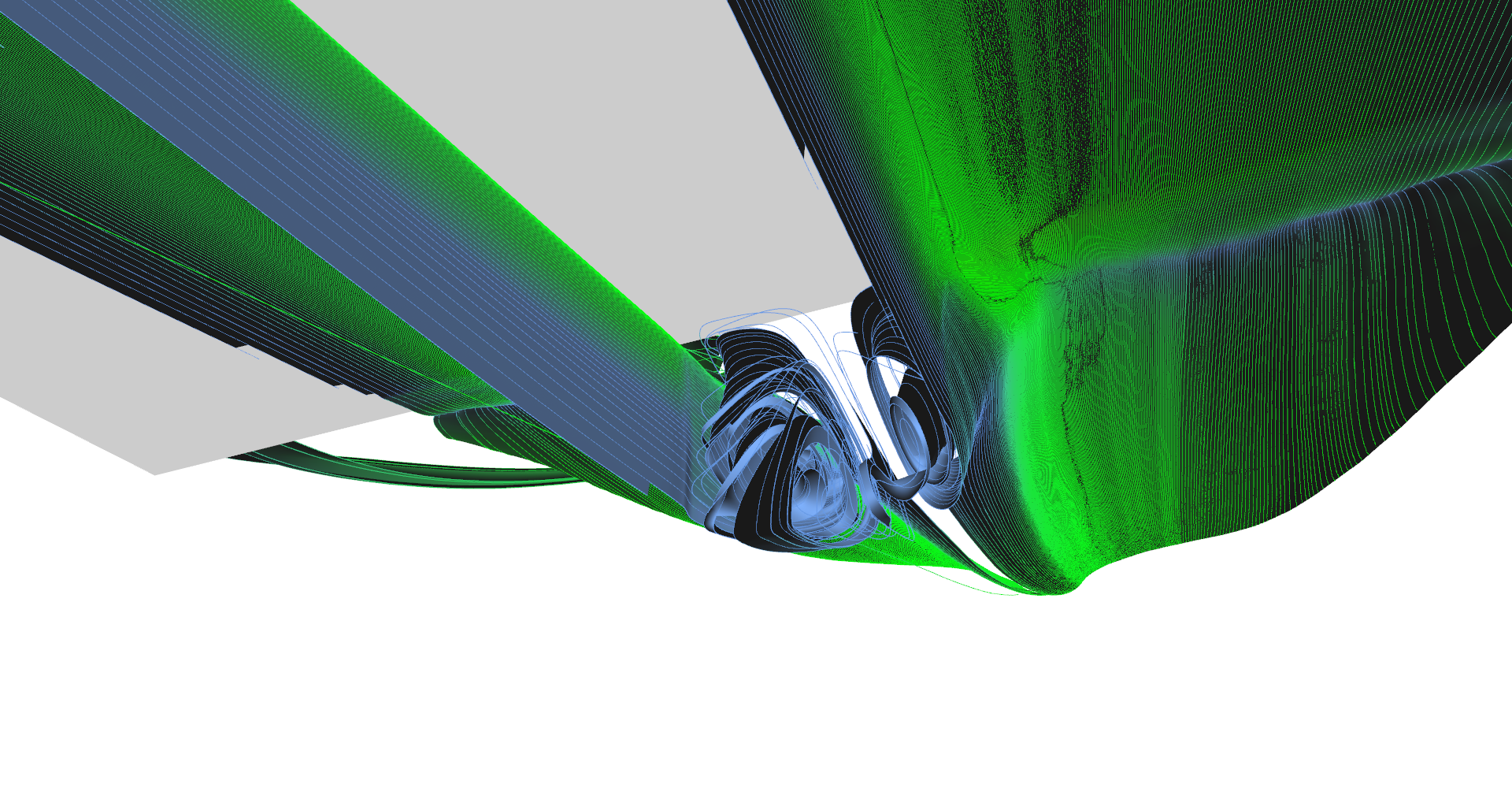
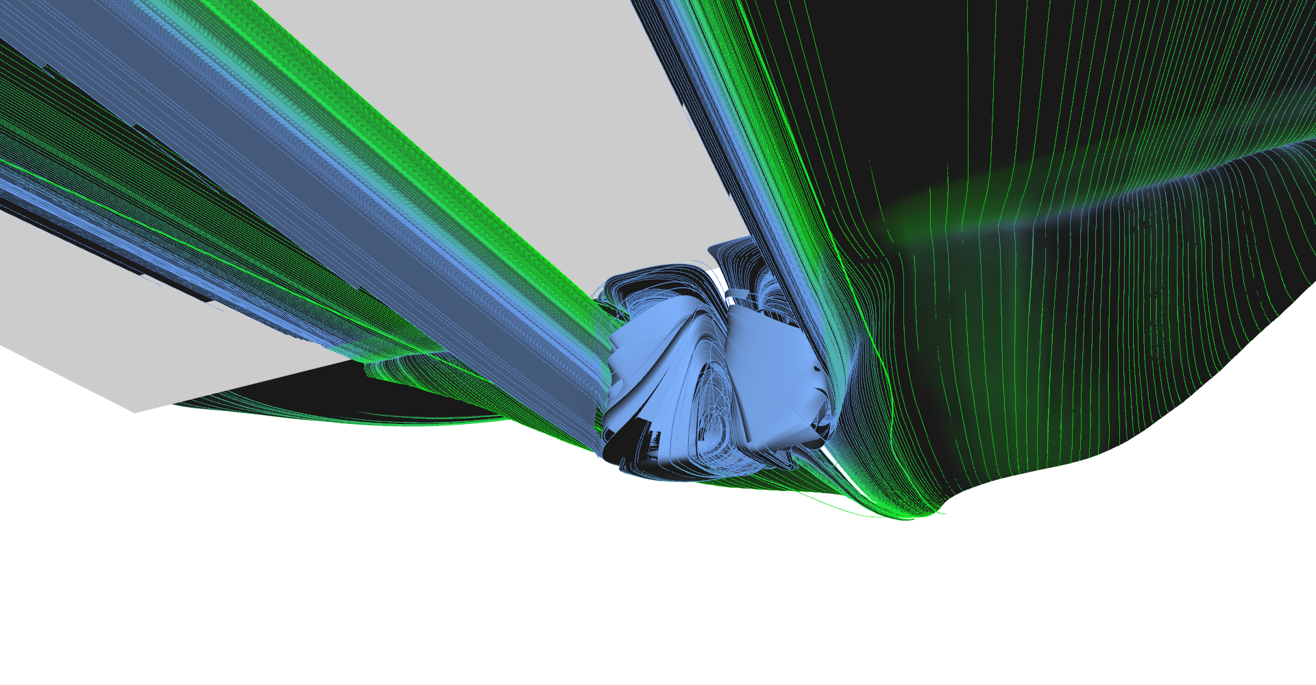
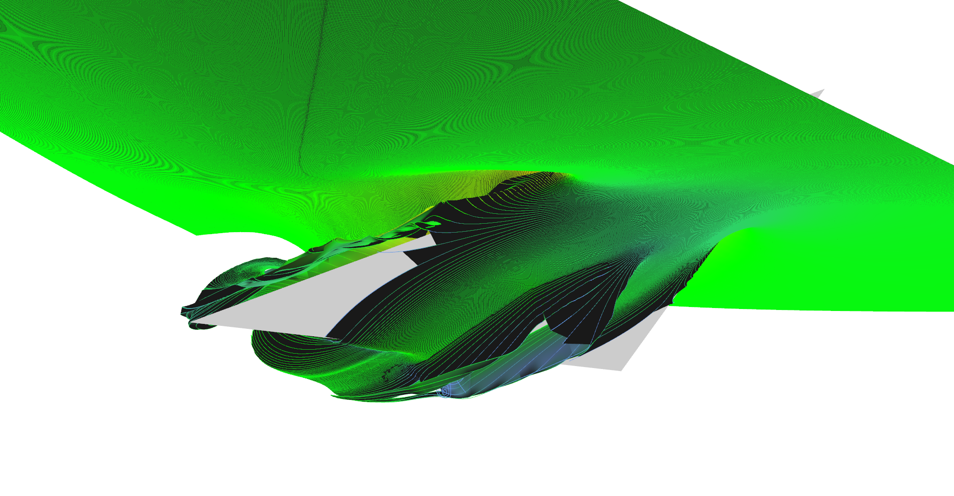
Adaptive line seeding was implemented with the hope that it will perform better than regular seeding with the same number of lines. Figure 17 shows wireframe mesh of both methods for comparison. Side-by-side comparison is shown in Figure 18 and I think that adaptive seeding does a better job than regular. However, nothing is for free, there is some performance drawback. Details about performance are in section 6: Performance benchmark. Please note again that I was not able to enable two-sided lighting model together with color material so one side of the surface is completely black.
Regularly seeded stream surface wireframe mesh Adaptively seeded stream surface wireframe mesh
Regularly seeded stream surface (pair 1) Adaptively seeded stream surface (pair 1) 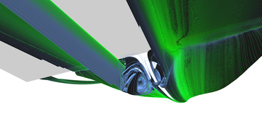
Regularly seeded stream surface (pair 2) 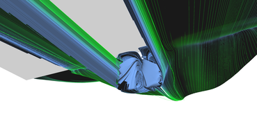
Adaptively seeded stream surface (pair 2) 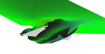
Regularly seeded stream surface (pair 3) 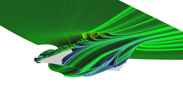
Adaptively seeded stream surface (pair 3)
6. Performance benchmark#
Most figures in this report were computed at interactive frame rates.
The biggest limitation of the CUDA approach is GPU memory.
Raw data itself consumed about 1.5 GB leaving about 2 GB for geometry.
The application has a parameter called geometry sampling which significantly lowers memory needed for geometry without losing integrator's precision.
Value of this parameter means how many samples of integrator to compute per sample of output geometry.
Another problem with memory is that all memory needs to be allocated before GPU kernel is invoked. This means that for every thread (potential line) there must be enough space no matter how long each stream line will be. If line integration stops in the middle there will be half of that line's memory unused.
In order to benchmark this application, time step was set to unnecessarily low values and number of primitives to ridiculous values.
Hardware#
Hardware matters since the solution is heavily using CUDA. The following hardware was used to create all figures in this report.
- OS: MS Windows 7 Enterprise 64-bit SP1
- CPU: Intel Core i7 920 @ 2.67GHz
- RAM: 12.0 GB Triple-Channel DDR3 @ 531MHz
- GPU: NVIDIA Quadro K5000, 4096 MB GDDR5
- CUDA Driver Version: 5.0
- CUDA Capability: 3.0 (program needs at least 2.0)
- 8 Multiprocessors x 192 CUDA Cores/MP: 1536 CUDA Cores
Comparison of Euler and RK4 integrators#
As discussed in section 3: Vector field integrators for stream line visualization,
I've implemented two different integrators.
Euler's integrator was implemented first because I thought that GPU is fast enough and smaller time step will ensure good precision.
In the middle of the project, one friend (math major) told me that RK4 would do much better than Euler no matter the time step.
For those who understand O-notation,
Euler's integrator has error O(dt2) and RK4 O(dt5) where dt is time step (dt << 1).
I did not believe them, so I implemented RK4 and compared results.
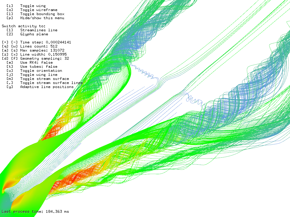
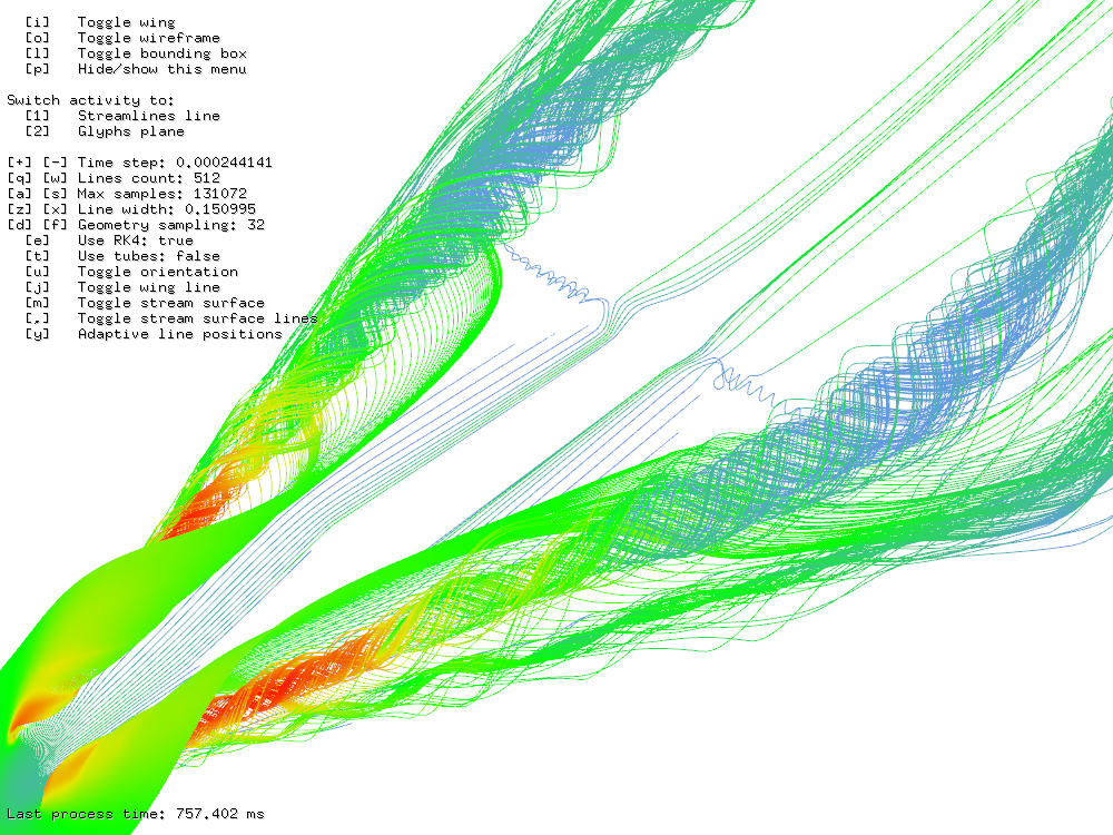
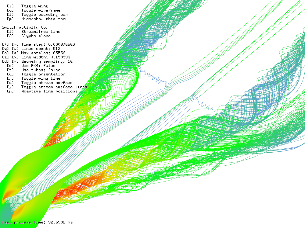
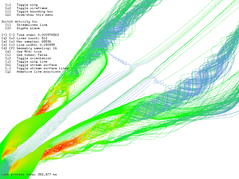
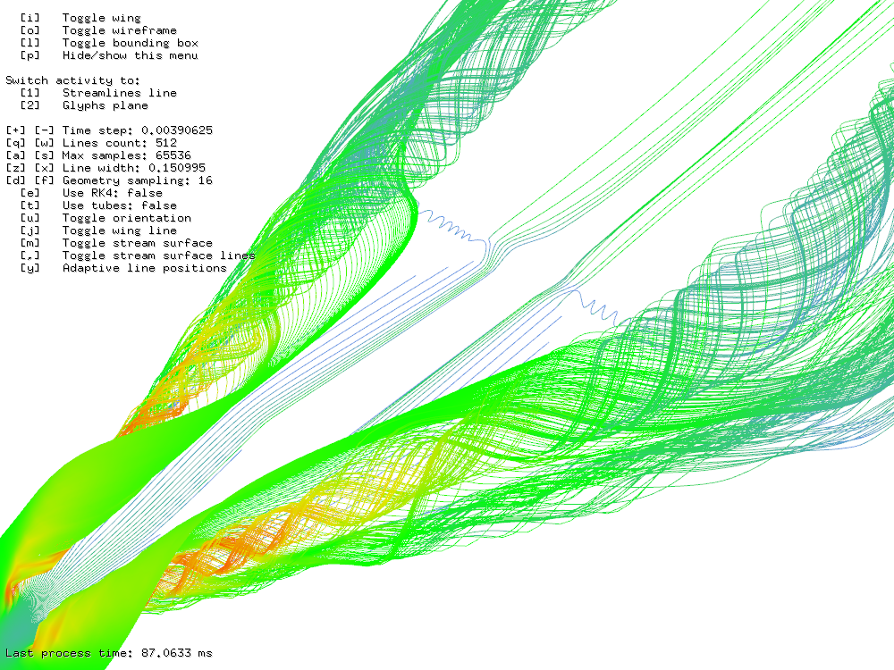
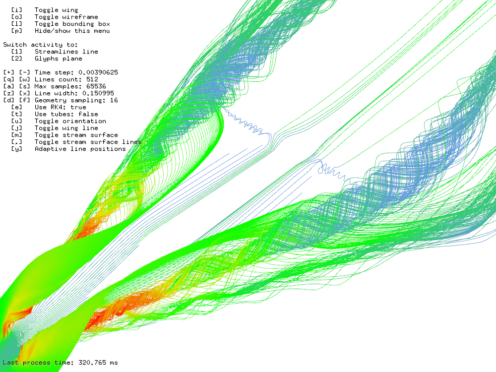
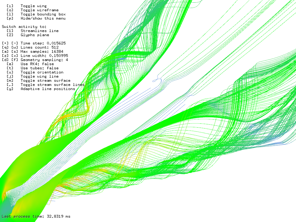
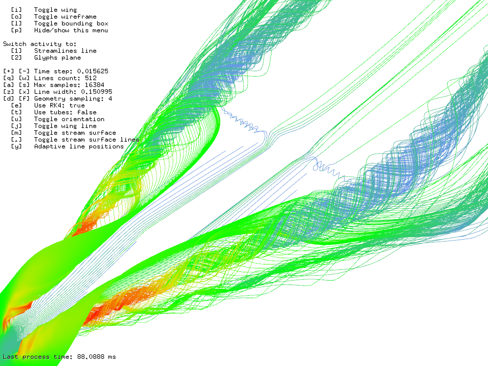
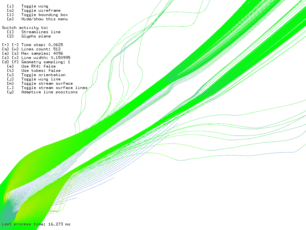
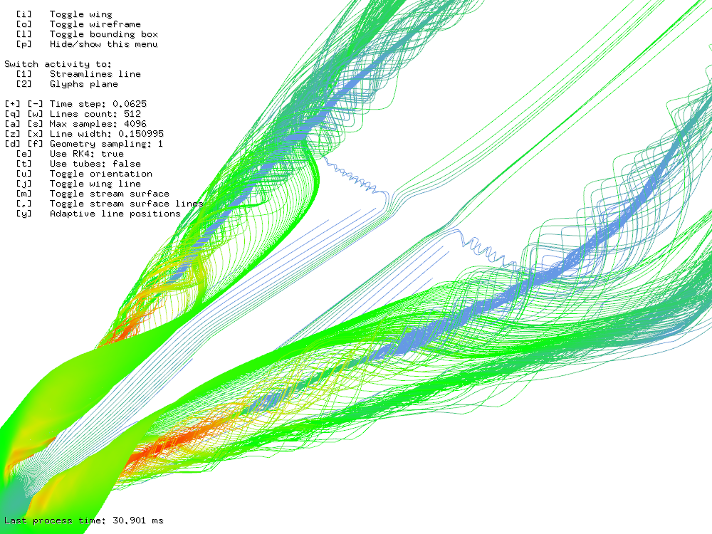
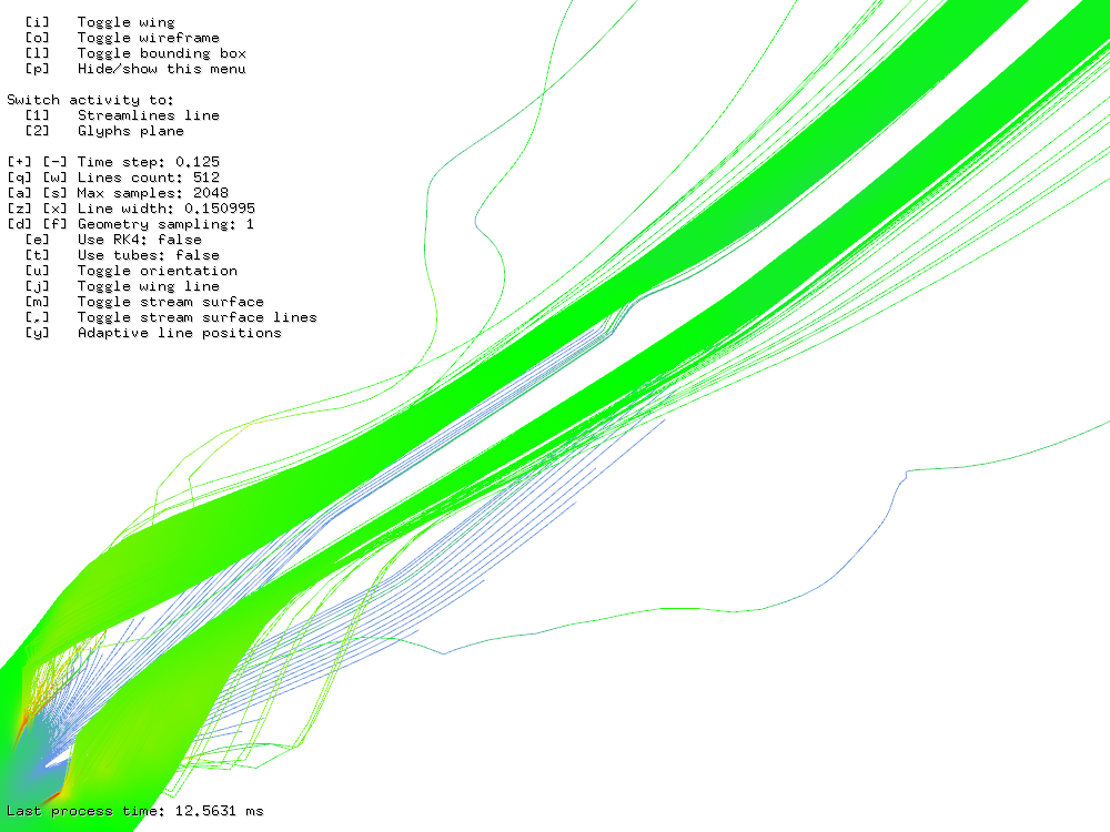
After comparing results visually (see Figure 19), I had to admit that my friend was right. Euler tends to escape vortices even for very low time step values but RK4 does a much better job. Interestingly enough, RK4 sometimes converges to the center of vortices instead of escaping them. I did not perform any measurement of the error because the visuals were enough for me to admit that RK4 does a much better job than Euler.
Euler integrator for dt=2^-12 
RK4 integrator for dt=2^-12 
Euler integrator for dt=2^-10 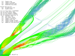
RK4 integrator for dt=2^-10 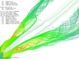
Euler integrator for dt=2^-8 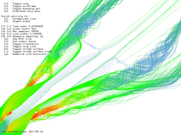
RK4 integrator for dt=2^-8 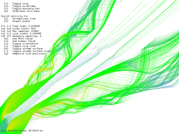
Euler integrator for dt=2^-6 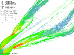
RK4 integrator for dt=2^-6 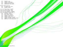
Euler integrator for dt=2^-4 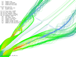
RK4 integrator for dt=2^-4 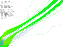
Euler integrator for dt=2^-3 
RK4 integrator for dt=2^-3
Glyphs#
The first benchmark was done with glyph lines. Since every line requires only one query to vector field, the number of lines literally does not matter at all. The only limit is GPU memory and every line takes very few of it as well. This means that the application is capable of rendering a huge amount of line glyphs at once. Figure 20 shows that nearly 13 million glyphs were computed in a mere 26 ms. The density of glyph lines is so high that you can even see individual voxels of data near edge of wing.
I did benchmark with arrow glyphs as well but the result was just a big blob of arrows and it was hard to see anything so I decided to not put the image here.
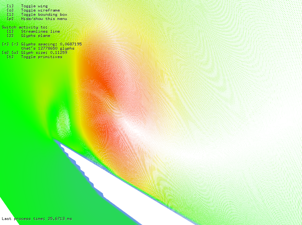 Figure 20: Nearly 13 million glyphs computed in 26 ms.
Stream lines and tubes#
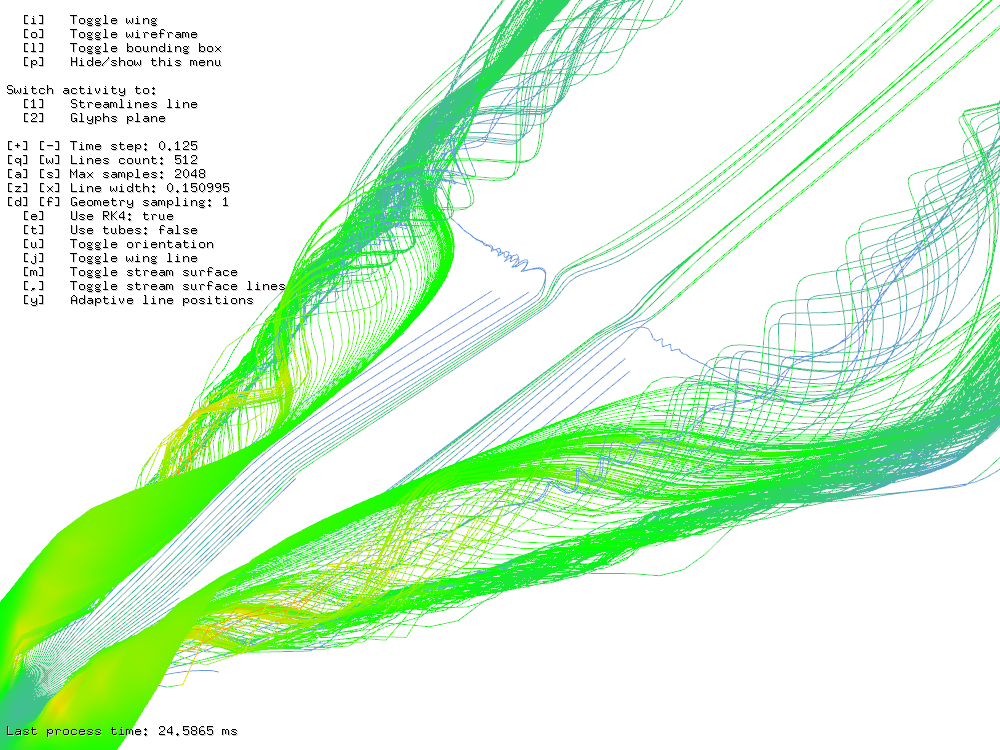
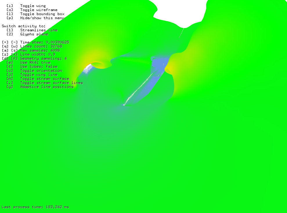
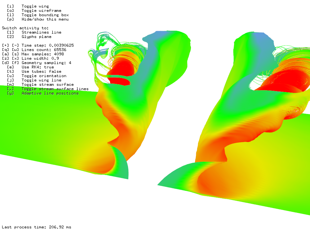
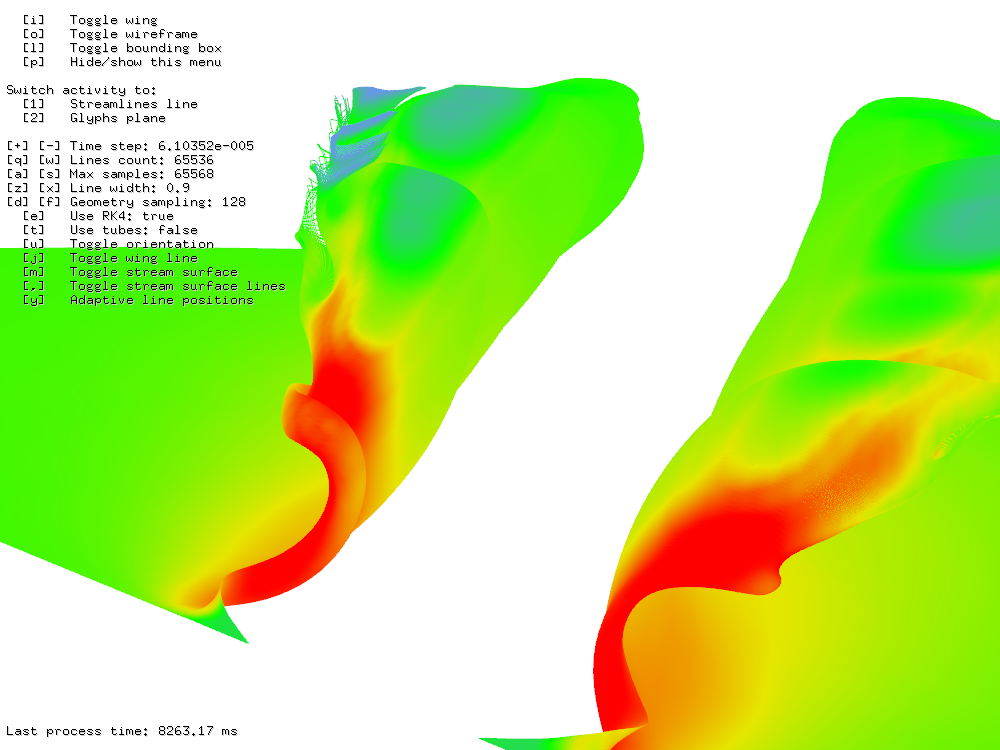
The second benchmark was dealing with stream lines. 215 stream lines for 212 steps took 183 ms and 216 stream lines took 207 ms. At this point the interactivity is not that great but 216 stream lines is just a crazy number anyway. Just for curiosity, 216 stream lines for 216 steps took a little more than 8 seconds. For this test I had to override the default time that Windows waits for the display driver to respond before it restarts it (default was 3 seconds).
215 stream lines for 212 steps took 183 ms. 
216 stream lines for 212 steps took 207 ms. 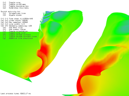
216 stream lines for 216 steps took 8 s.
The third benchmark uses an adaptive algorithm for computing stream lines. As you can see in Figure 22 it is roughly three-times slower computing 215 stream lines for 212 steps in 450 ms. However if you take into account that the adaptive algorithm is counted in an iterative manner on GPU and CPU, the result is surprisingly fast.
Unfortunately, the adaptive algorithm does not work with stream tubes. There is a bug that stream lines are all over the place - some array indices get messed up while counting adaptive algorithm and I had no time to fix it.
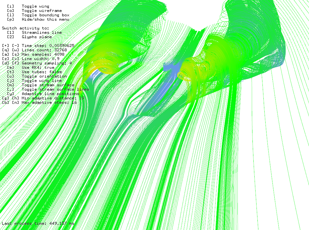 Figure 22: 215 stream lines for 212 steps using adaptive algorithm took 450 ms.
The next benchmark was testing stream tubes. Computation power needed for integration of stream tubes is the same as for stream lines but stream tubes have much more vertices and the kernel also computes indices for faces and normals which makes them heavy for memory writing and consumes much more overall GPU memory. Figure 23 shows that 213 stream tubes of 213 samples took 240 ms.
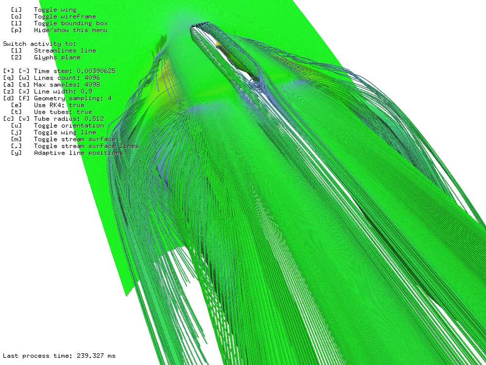 Figure 23: 213 stream tubes for 213 steps took 240 ms.
Stream surface#
The last test is testing adaptive stream surface algorithm. Figure 24 shows that 213 seeds for 212 steps using adaptive stream surface algorithm took 532 ms.
Because of the adaptivity of the algorithm total time depends on the origin of the stream surface. However, my goal was not to do scientifically precise proof but just to estimate what my system is capable of.
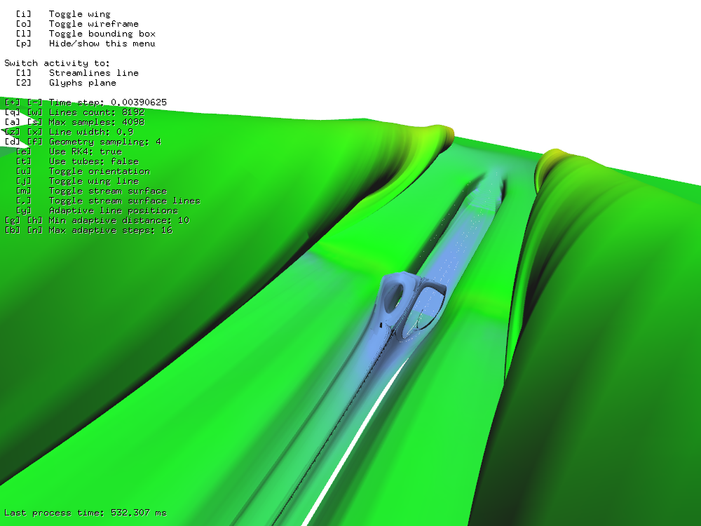 Figure 24: 213 seeds for 212 steps using adaptive algorithm took 532 ms.
Extra#
Lastly, Figure 25 shows SysInternal's Process Manager GPU card while I was playing with the program. GPU is not 100% utilized because there is always some spare time between CUDA individual computations.
It was quite interesting to observe how the operating system and nVidia drivers handle situations when GPU is out of memory. Sometimes, part of GPU memory was swapped and "GPU System Memory" graph rose. Unfortunately, usually the application just failed to allocate GPU memory. I was not able to achieve any stable results.
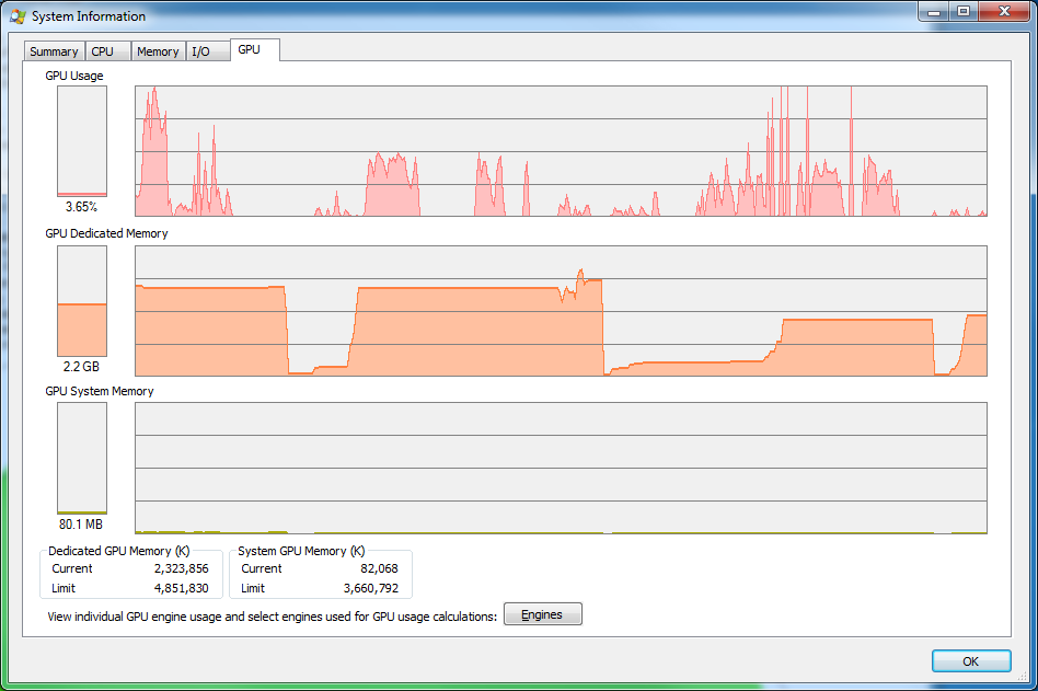 Figure 25: Process Manager GPU card while working with the program.
7. Conclusion and downloads#
I really enjoyed this project and I learned a lot about vector fields as well as about CUDA. This project went far beyond course requirements and I received 100/100 from the project and an A from the class.
The downside of the application itself is the fact that you need to have somewhat recent NVIDIA GPU in order to run it. The code was developed and tested only on Windows using delta-wing dataset. To run the application might require CUDA installed. Test dataset can be downloaded below.
If you are interested in the implementation please see the code on GitHub.
Download
- DeltaWing-LowestResolution.7z — Low-resolution dataset of delta-wing vector field.