Maraytr - Marek's Ray-tracer

Maraytr is a ray-tracer written with high focus on algorithms and data structures rather than on performance. I decided to make it to get deeper understanding of theory and math behind ray-tracing. Also, ray-tracing is fun! The core was written in four days in C# without any third-party libraries. The scene is represented as Constructive Solid Geometry (CSG) and supported primitives are sphere, cube, and plane. It is possible to do basic boolean operations like union, intersection, subtraction, or xor.
Source code is available on GitHub: NightElfik/Maraytr

A dice created from cubes and spheres using boolean operations. 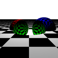
Result after second day of work. 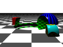
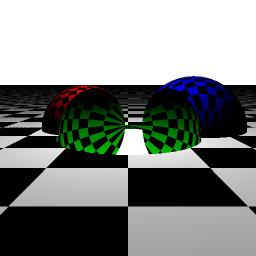
Result after third day of work. 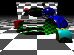
Result after fourth day of work. 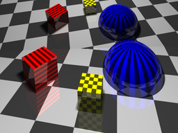
Example of reflections. 
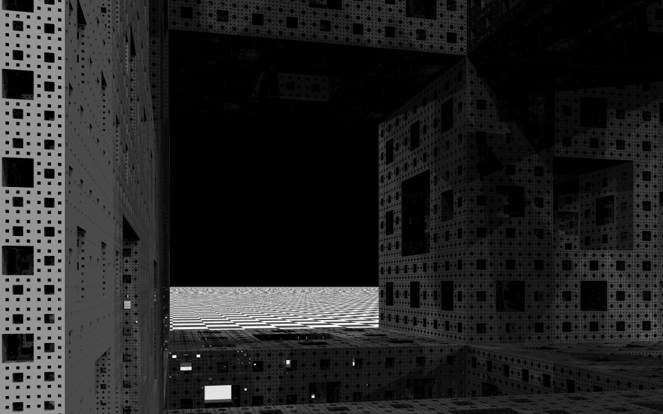
Procedurally generated Menger sponge (8th iteration).
Introduction
One day I have decided that I want to write a ray-tracer. I have been taught in school a lot of theory but I have never written a ray-tracer from scratch.
This report is not meant to be a step-by-step tutorial how to make a ray-tracer but rather explanation of features and design decisions of my implementation. However, this article offers a good overview of core functionalities and can serve as an inspiration for your own implementation. I believe that a step-by-step guide is actually not that useful and solving problems by your own (with hints) is the best way to learn.
Scene representation
The first decision should be made about representation of a scene. There are two main options to consider.
The first option is represent the scene as a bunch of triangles — triangle mesh. This representation is quite convenient, ray-triangle intersection algorithm is simple, and you will be able to download 3D models from internet and load them into your program. The problem is that creating your own shapes is not easy and boolean operations such as intersection and subtraction are hard. Also, texturing is a problem.
The second option is to represent shapes purely procedurally, for example as sphere defined only by center and radius. An example of such scene is shown in Figure 2. Based on this little information one can write a function that computes an intersection between ray and sphere. And the sphere will be mathematically perfect. The advantage of this representation might be ability to do boolean operations easily and procedural texturing is also simple. The biggest disadvantage is that making more complicated shapes is very hard. You have to construct them only using primitive shapes and boolean operations.
Figure 2: A procedurally created scene containing spheres, cubes, and planes. More complicated shapes are created using boolean operations. The mirror in the back is just a plane intersected with a box and it has 100% reflectivity. Notice the soft shadows and reflection on the blue sphere.Constructive solid geometry
I have decided to represent the scene procedurally because it is in my eyes much cooler and also there are more things to play with. However, the design allows to add triangle meshes support without problems later.
A good way to represent procedural scene is Constructive solid geometry. CSG can be represented as a binary tree where leaves are primitives and internal nodes are operations. Every node have also information about its relative transformation such as rotation or translation. The trick is that the transformation is applied on the ray rather than on the object. This trick can dramatically reduces complexity of intersection functions (more on that later in section CSG primitives).
CSG is actually quite powerful representation because it is volumetric representation. It is used by come CAD programs for designing real-world objects. The more primitive objects you have the more complicated things you can create with them.
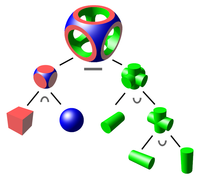 Figure 3: CSG objects represented as a binary tree. The ∩ is intersection, ∪ is union, and — is difference (by Zottie from Wikipedia)
The scene class shown in Code listing 1 contains basic information such as the scene root, camera, and lights. Everything is defined through interfaces to enable easy extensibility.
The scene root can be anything that can be intersected. In our case it will be the node (root) of CSG tree but it is possible to write a class that intersects triangle meshes or anything else.
1
2
3
4
5
6
7
8
9
10
11
public class Scene {
	public IIntersectable SceneRoot { get; set; }

	public ColorRgbt BgColor { get; set; }
	public IReflectionModel ReflectionModel { get; set; }

	public ICamera Camera { get; set; }

	public ColorRgbt AmbientLight { get; set; }
	public List<ILightSource> Lights { get; set; }
}
CSG primitives
The key elements in the CSG representation are primitive shapes. The cool part is that every shape is defined algorithmically by its intersection procedure. Just think about it, there is no actual sphere in the scene, just a piece of program that is able to compute if given ray intersects it or not.
Wait, and how about center and radius?
Good question, but nope, we don't need those. As already mentioned, every node in CSG graph contains its transformation. If your intersection method is written to intersect unit sphere with center in origin then you just translate and scale it to get any general sphere. Isn't this cool? All the very basic shapes does not need any information — just the intersection function.
Talking about intersection functions, let's derive the one for a sphere.
For the notation, bold symbols are 3D vectors, normal symbols are just scalars.
A sphere with center c and radius r
can be defined as (x - c)2 = r2.
The equation can be interpreted as all points x with distance r from point c.
A ray starting in point s going in direction d
is a set of points x for which x = s + t∙d.
The direction d is unit vector and t is time parameter that specifies a position among the ray.
Now we just put the two equations together while setting c = 0 and r = 1.
(x - 0)2 = 12x = s + t∙d(s + t∙d)2 = 1s∙s + 2 t s∙d + t2 d∙d = 1d is unit vector so d∙d = 1
t2 + t (2∙s∙d) + (s∙s - 1) = 0t.
D = B2 - 4 A C, where Ais 1,Bis 2∙s∙d, andCis s∙s - 1.
D = 4∙(s∙d)2 - 4∙s∙s + 4t1,2 = -B ± D0.5 / 2∙A t1,2 = -s∙d ± ((s∙d)2 - s∙s + 1)0.5 = -s∙d ± (D / 4)0.5a∙b is dot-product: a∙b = Σi ai ∙ bi
Equation 9 gives us the solution in terms of two numbers t.
We can compute a point of intersections using original ray equation x = s + t∙d.
If t is negative then the intersection is in behind us
(in opposite direction than direction vector d).
Understanding the math underneath is crucial. For example, we ended up with two solutions, why? Because a ray can intersect a sphere at two points. That makes sense, right?
The math also gives us a hint about some special cases.
For example, when D is negative we cannot compute its square root.
That actually mean that the ray missed the sphere and there are no intersections.
When D is zero then the ray is tangent to the sphere and we have only one intersection.
Turning the math into the code is very simple as you can see in Code listing 2. The only catch is the case with one intersection. We want to have either two intersections or none because intersection represents entering and leaving the volume of the object. So I consider (near) tangent ray as a miss (section CSG operations explains why having intersections paired is important).
Other primitives such as cube and plane are described in similar way. Now we are ready to start shooting some rays!
1
2
3
4
5
6
7
8
9
10
11
12
13
14
15
16
17
18
19
20
public class Sphere : IIntersectableObject {
	public int Intersect(Ray ray, IList<Intersection> outIntersections) {
		double sd = ray.StartPoint.Dot(ray.Direction);
		double ss = ray.StartPoint.Dot(ray.StartPoint);

		double discrOver4 = sd * sd - ss + 1;
		if (discrOver4 <= 0.0 || discrOver4.IsAlmostZero()) {
			return 0;  // 0 or 1 solution, but we want two.
		}

		double discrOver4Sqrt = Math.Sqrt(discrOver4);
		double tEnter = -sd - discrOver4Sqrt;
		double tLeave = -sd + discrOver4Sqrt;
		Debug.Assert(tEnter < tLeave);

		outIntersections.Add(new Intersection(this, true, ray, tEnter));
		outIntersections.Add(new Intersection(this, false, ray, tLeave));
		return 2;
	}
}
Transformations
The binary tree structure of the CSG representation also allows to conveniently store transformations. Every node stores a relative (local) transformation from its parent as affine transformation matrix.
Code listing 3 shows CSG node class.
Every node has reference to its parent, list of children and a local transformation.
The Intersect method have to be implemented by derived class.
There are two derived classes: the one representing geometric primitives (leaves) and then the boolean operation nodes (internal nodes).
The primitives just compute the intersection with given ray.
Interesting stuff happens in the operation nodes and will be described later in section CSG operations.
1
2
3
4
5
6
7
8
9
10
11
12
13
14
15
16
17
18
19
20
public abstract class CsgNode : IIntersectable {
	public CsgNode Parent { get; set; }
	public bool IsRoot { get { return Parent == null; } }

	protected List<CsgNode> children = new List<CsgNode>();
	public IEnumerable<CsgNode> Children { get { return children; } }
	public bool IsLeaf { get { return children.Count == 0; } }
	public int ChildrenCount { get { return children.Count; } }

	public Matrix4Affine LocalTransform { get; set; }

	public abstract int Intersect(Ray ray, IList<Intersection> outIntersections);

	public virtual void PrecomputeTransformCaches(Matrix4Affine globalTransform) {
		var t = globalTransform * LocalTransform;
		foreach (var child in children) {
			child.PrecomputeTransformCaches(t);
		}
	}
}
Ray caster
Now that we know how the scene is represented let's quickly talk about how intersections are computed and then we can finally cast some rays!
Intersections computation
As described in section CSG primitives the ray intersection method of primitive shapes has no information about position, scale, or rotation of the object.
Instead of moving the object itself we move the rays.
In order to transform a ray from global coordinate system to local one we have to apply all transformations from current node to the root.
It is wasteful to do this costly operation for every ray so method PrecomputeTransformCaches in
CsgNode and CsgObjectNode classes pre-computes the transformations.
Transformations and matrix multiplications can be tricky and you may have to spend more time to understand them. I will mention just a few tips here.
First, you have to apply inverse of the object transformation on rays. Imagine this as shooting at a target. Instead of moving the target to the right and hitting left side of it you can leave the target in place and move yourself to the left (opposite of moving the target right).
Second, the order of multiplication is significant. Basically you want to apply the top level inverse first and then continue down in the tree. That's the same as applying the bottom level direct transformation first, keep multiplying all the way to the root, and then take inverse of the whole thing (that is how it I did it in the code). In math words:
T2-1 ∙ T1-1 ∙ T0-1 ∙ v = (T0 ∙ T1 ∙ T2)-1 ∙ v
The top level inverse transformation T0-1 is applied to the vector v first, then T1-1, and finally T2-1.
I assume that all vectors are multiplied from the right side of the matrix.
If you multiply vectors from the left side, everything is reversed.
Understanding transformations is crucial and if you find yourself struggling with them then I highly suggest digging deeper into this topic on your own. The worst think you can do is the trial-error approach — guessing the matrix multiplication order and inverting vs. not inverting, etc. I have written the code without any trials. It worked on the first try (more or less :).
1
2
3
4
5
6
7
8
9
10
11
12
13
14
15
16
17
18
19
20
21
22
23
24
25
26
27
28
public class CsgObjectNode : CsgNode, IIntersectableObject {
	public IIntersectableObject IntersectableObject { get; set; }
	public IMaterial Material { get; set; }

	private Matrix4Affine globalToLocalTransformCache;
	private Matrix4Affine localToGlobalTransformCache;

	public override void PrecomputeTransformCaches(Matrix4Affine globalTransform) {
		localToGlobalTransformCache = globalTransform * LocalTransform;
		globalToLocalTransformCache = localToGlobalTransformCache.Inverse();
	}

	public override int Intersect(Ray globalRay, IList<Intersection> outIntersections) {
		int startIndex = outIntersections.Count;
		Ray localRay = globalRay.Transform(globalToLocalTransformCache);
		int isecCount = IntersectableObject.Intersect(localRay, outIntersections);

		for (int i = 0; i < isecCount; ++i) {
			var isec = outIntersections[startIndex + i];
			isec.IntersectedObject = this;
			isec.Position = localToGlobalTransformCache.Transform(
				localRay.GetPointAt(isec.RayParameter));
			isec.RayDistanceSqSigned = (isec.Position - globalRay.StartPoint)
				.LengthSquared * (isec.RayParameter >= 0.0 ? 1 : -1);
		}
		return isecCount;
	}
}
Camera
Camera is a source of rays. The very basic orthographic camera just shoots parallel rays from a rectangle in 3D space. The rectangle is basically the camera and it shoots one ray per pixel. Code listing 5 shows interface of any camera class. As you can see it converts x-y screen coordinate to a ray.
1
2
3
4
public interface ICamera {
	Size Size { get; set; }
	Ray GetRay(double x, double y);
}
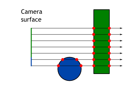
Orthographic camera is boring. Better is perspective camera and it is actually not that complicated. The difference is that rays are not parallel but they form a frustum — a pyramid with the tip chopped off. The tip is where the rays are originated. Figure 4 shows simple example of both camera models.
I will not go over the details here but I will give just a few hints. Camera does not need to have a position or direction of look. Those can be hard coded, for example camera can be in the origin and point in the x direction. Instead of moving the camera you can move the scene in front of it.
Another hint is that angles between individual rays in perspective camera are the same.
However, be careful that you have to bend them in X and Y direction as well.
Simple way is to compute angle increment as field of view/width in px
and then use that increment for the other axis as well.
In case of troubles feel free to check the code.

Orthographic camera. 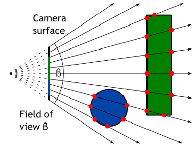
Perspective camera.

Ray casting
Now we have rays associated to every pixel of result image and we are able to compute intersections. By putting those two steps together we have a simple ray-caster (not ray-tracer yet).
Code listing 6 shows basic structure of the Intersection class.
Every intersection stores information about the ray, ray parameter t, if it is entering or leaving ray,
and some other things that will be discussed later.
1
2
3
4
5
6
7
8
9
10
11
12
13
14
15
16
public class Intersection : IComparable<Intersection> {
	public IIntersectableObject IntersectedObject;

	public Ray Ray;
	public double RayParameter;
	public bool IsEnter;
	public bool InverseNormal;

	public Vector3 Position
	public double RayDistanceSqSigned;
	public Vector3 Normal;

	public Vector2 TextureCoord;
	public IMaterial Material;
	public object AdditionalData;
}
For every ray tries to intersect all objects in the scene and gather a list of intersections. Then simply discard all that have negative ray parameter because they are behind the camera. Now you can display white pixel if there are some intersections and black if they are not. You should see something similar to Figure 5.
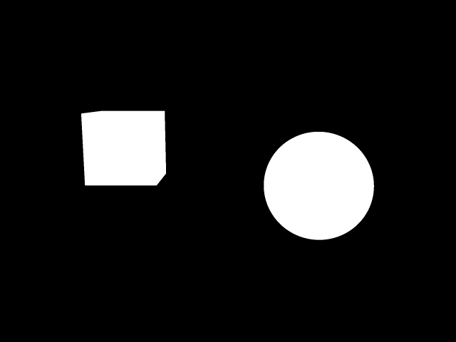 Figure 5: Result of putting white pixel for intersection and black for no intersection.
Colors and textures
Black and white is not fun.
Let's add some colors!
If we look at the list of intersections for every ray we can choose the intersection which is closest to its origin.
That's the one with the smallest positive ray parameter t.
Now we can display a color based on the object which was hit.
We know that because it is saved in the Intersection class.
Figure 6 shows how a simple scene might look like.
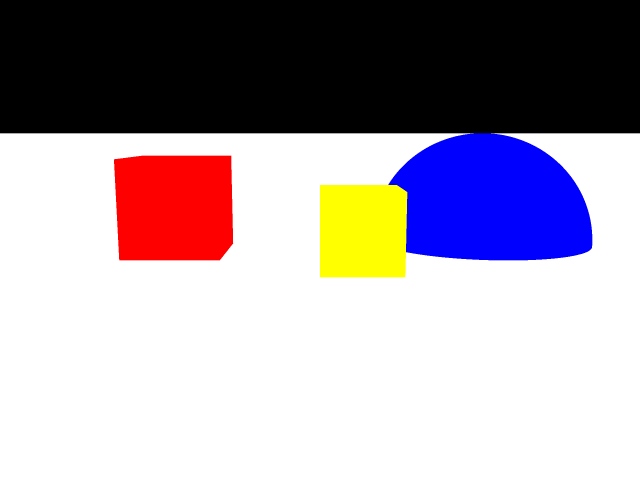 Figure 6: Color based on the closest hit of the ray.
Procedural textures are also simple. For 2D textures we have to compute texture coordinates. A texture coordinate is a 2D position on the surface. For a plane that's just position of the intersection. For a sphere it can be defined as longitude and latitude. Texture coordinates are usually defined from 0 to 1.
As an example Code listing 7 shows computation of texture coordinates on the sphere.
They are computed in the CompleteIntersection method on the primitive object.
We do not need to compute texture coordinates or normals for all intersections.
Only the ones that are being used and displayed need the additional data.
As an optimization the intersections are first filtered and then additional data is computed.
1
2
3
4
5
6
7
8
9
10
public class Sphere : IIntersectableObject {
	public void CompleteIntersection(Intersection intersection) {
		Vector3 localIntPt = intersection.LocalIntersectionPt;
		intersection.Normal = localIntPt;

		intersection.TextureCoord.X = Math.Atan2(localIntPt.Z, localIntPt.X)
			/ (2.0 * Math.PI) + 0.5;
		intersection.TextureCoord.Y = Math.Atan2(1, localIntPt.Y) / Math.PI;
	}
}
Based on the texture coordinate we can do some simple shapes like stripes or checkers. Just for completeness the code for checkers is in Code listing 8.
You might be asking: Can I use the 3D coordinate for some kind of 3D texture?
The answer is yes, of course!
It is maybe even simpler to do volumetric checkers, stripes or dots.
As you can see the texturing method has access to the Intersection class
so you can even use normal or ray parameter to do textures based on those!
I am just sticking with traditional 2D textures for now.
1
2
3
4
5
6
7
8
9
10
11
12
13
14
15
16
17
public class CheckerTexture2D : ITexture {
	public double UFrequency { get; set; }
	public double VFrequency { get; set; }

	public ColorRgbt EvenColor { get; set; }
	public ColorRgbt OddColor { get; set; }

	public ColorRgbt GetColorAt(Intersection intersection) {
		double u = intersection.TextureCoord.X * UFrequency;
		double v = intersection.TextureCoord.Y * VFrequency;

		long ui = (long)Math.Floor(u);
		long vi = (long)Math.Floor(v);

		return ((ui + vi) & 1) == 0) ? EvenColor : OddColor;
	}
}
Example scene with textured objects is show in Figure 7. Thanks to the textures you can see the perspective and the objects much better even though there are no lights and shadows in the scene.
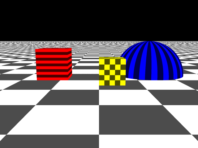 Figure 7: Example of simple scene with textures.
Ray tracer
Turning ray-caster to ray-tracer is done by adding secondary rays that are able to compute shadows and reflections.
Lights and shadows
The simplest light is a point light because from any point you either see it or not. Point light casts hard shadows. Computing whether a point is lit by a point light is very simple — just cast a ray from the point to the light. If the ray hits anything then the original point is in shadow. Otherwise we can compute light intensity based on the distance and normal angle. I use basic Phong reflection model for that. Example of one point light in a scene is in Figure 8
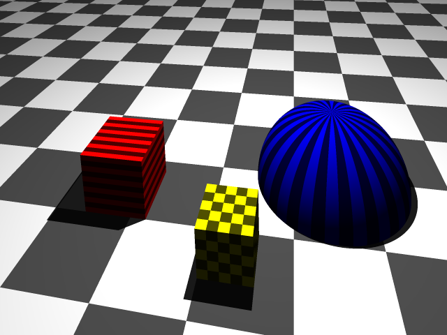 Figure 8: Example of simple scene a point light casting hard shadows.
Area lights are usually simulated as an array of point lights. For every pixel we have to cast multiple rays to all point lights in area light source.
This is starting to be very computationally expensive.
To lower the load it is possible to connect light sampling with sub-pixel sampling
(this technique is called Super-sampling).
Say, we are casting 16 sub-pixel rays per pixel to make the result image smooth.
In the scene we have an area light that is made of also 16 point lights.
Now to compute lighting for every pixel we need 16∙16 = 256 rays.
However, we can combine the two integrations together and send sub-pixel-ray number i to
only one sub-point-light number i (not to all of them).
This will result in only 2∙16 = 32 rays.
This is why you can find IntegrationState information passed to the light source.
Figure 9 shows area light with described optimized sampling technique. You can see shadow artifacts from roughly four levels. This is because the area light is 4x4 point lights perfectly aligned in a grid. The artifacts can be reduced by using jittering.
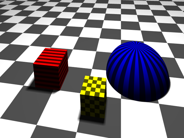 Figure 9: Example of area light casting (somewhat) soft shadows.
Reflections and refractions
Reflections (and refractions) are little more complicated than lights. Refractions are very similar to reflections and I will describe only reflections here.
Every object has to have information about how much reflective it is.
This information is accessible through ReflectionFactor property in IMaterial (Code listing 9).
Now the real ray-tracing begins.
1
2
3
4
5
public interface IMaterial {
	ColorRgbt BaseColor { get; }
	ITexture Texture { get; }
	float ReflectionFactor { get; }
}
First a primary ray is casted and intersection is obtained. Then, secondary ray is cast if the reflection factor is greater than a limit (close to zero). The direction of reflected ray is given by standard reflection model based on the surface normal. The ray may be bouncing many times around the scene. The important thing is to keep track of total contribution and stop the bouncing if the contribution is too low. For example, imagine two 50% mirrors. First bounce will have 50% contribution, second 25% (50% of 50%), third 12.5% (50% of 25%), etc. Sum of all colors multiplied by their contributions gives the final color.
Recursion provides a great way to achieve this process. Code listing 10 shows the method that computes the described ray-tracing. This is a core of the ray-tracer.
1
2
3
4
5
6
7
8
9
10
11
12
13
14
15
16
17
18
19
20
ColorRgbt traceRay(Ray ray, IntegrationState intState, int depth, double contribution) {
	var isec = getIntersection(ray);
	if (isec == null) {
		return scene.BgColor;
	}

	ColorRgbt color = evaluateIntersection(isec, intState);

	contribution *= isec.Material.ReflectionFactor;
	if (depth >= MaxTraceDepth || contribution < MinContribution) {
		return color;
	}

	Vector3 reflectedDir = computeReflection(isec.Normal, -ray.Direction);
	reflectedDir.NormalizeThis();

	ColorRgbt reflectedColor = traceRay(new Ray(isec.Position, reflectedDir),
		intState, depth + 1, contribution);
	return color + reflectedColor * isec.Material.ReflectionFactor;
}
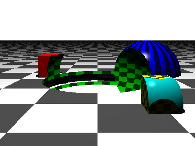
The result of reflections is show in Figure 10. The floor has 50% reflectance and all the objects have 30%. The cool thing about reflections is that you can put mirrors in the scene! The mirror in the back of the image has 95% reflectivity and it is tilted in X and Y directions by 10 degrees.
If you look carefully you can see that the yellow cube in front has much worse soft shadow than the red cube. This is caused by not using jittering on the area lights. The samples of the area light are aligned with the yellow cube. Due to the sampling you can see four intensities because the light is made of 4x4 point lights. The red cube is rotated by 30 degrees which result is much smoother shadow.
 Figure 10: All objects in this scene are reflective. There is a huge mirror in the back of the scene.
Extensions
The basic ray-tracer was described in previous chapters. In this chapter I will go over some extra features. I might add new sections over time as new features will be i
CSG operations
The cool part about CSG representation is ability to do boolean operations. The basic idea is to collect intersections from all children and filter them based on the boolean operation. I will describe here only union and intersection, others are similar. Figure 11 shows the process visually.
Note that in order to perform boolean operations correctly all intersections has to be paired. For every enter intersection has to be another exit intersection. This is why we ignored tangent intersection with the sphere in section CSG primitives . This may be tricky to fulfill with objects like half-space tha have only one intersection. I solve it by adding extra intersection that is in infinity.
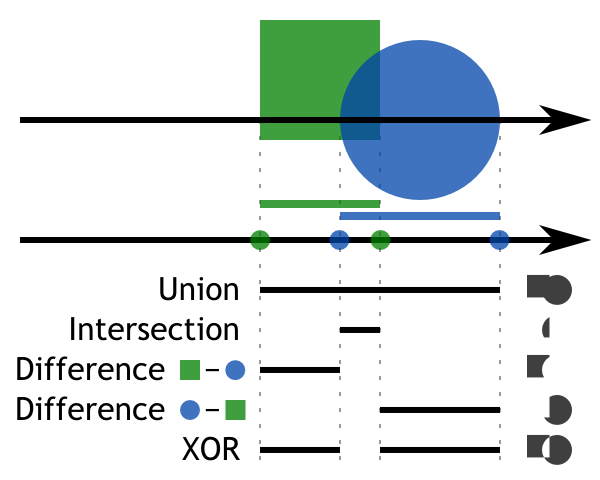 Figure 11: Visual explanation of boolean operations among one ray based on intersections.
The magic happens in the Intersect method of CsgBoolOperationNode.
All intersections are collected to a list which is then sorted by the ray parameter.
Now we have a list of intersections that comes how they appear among the ray.
We will go through them one by one and produce new pruned list of intersections based on a boolean operation of the node.
For union, at least one object has to be present. For intersection all child object have to be present. We will keep track of number of objects we are currently in. Every enter intersection will increase the counter and every leave intersection will decrease it.
Now for the union, when counter increases from zero to one we save that intersection. If counter decreases from one to zero we again save the intersection. All other intersections will be not saved to the final list.
Intersection works the same but the reporting threshold is not one but n which is the number of children.
Code listing 11 shows the code that performs described operation.
The parameter requiredObjectsCount is one for union and n for intersection.
This method can perform partial intersection where say only two overlapping objects are needed to satisfy intersection condition.
I can imagine this partial intersection be used when having a long chain of spheres and every two are overlapping a little bit.
1
2
3
4
5
6
7
8
9
10
11
12
13
14
15
16
17
18
19
20
21
22
23
24
25
int computeIntersection(List<Intersection> intersections,
		ICollection<Intersection> outIntersections, int requiredObjectsCount) {
	int insideCount = 0;
	int count = 0;

	foreach (var intersec in intersections) {
		if (intersec.IsEnter) {
			++insideCount;
			if (insideCount == requiredObjectsCount) {
				outIntersections.Add(intersec);  // Add entering intersection to the result.
				++count;
			}
		}
		else {
			if (insideCount == requiredObjectsCount) {
				outIntersections.Add(intersec);  // Add leaving intersection to the result.
				++count;
			}
			--insideCount;
		}
	}

	Debug.Assert(insideCount == 0);
	return count;
}
I have created simple dice as an example of boolean operations (see Figure 12). The basic shape is an intersection of cube and sphere. Then corers are cut using cubes of size little smaller than diagonal of the main cube. Finally, small black spheres are used to cut the holes using subtraction operation.
This scene does not use ambient light. The shadowed are on the right side of the dice is lit by very soft blue-ish point light. If you look carefully you can see a shadow from it on the left side.
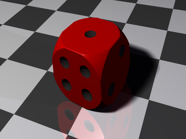 Figure 12: A dice created from cubes and spheres using boolean operations.
Conclusion
Everyone who is serious about computer graphic should write their own ray-tracer. From scratch! It is a great way how to deeply understand many aspects of computer graphics such as transformations and color theory. Ray-tracer is also great line for resume.
Code
You can find full source code published under Public Domain on the GitHub.