Realtime visualization of 3D vector fields using CUDA

Chapter 3: Vector field integrators for stream line visualization

Before we jump in visualization techniques using stream lines and stream surfaces I would like to mention implementation details of used integrators.

Stream line is trajectory of mass-less particle in vector field. Integrators are used to simulate this trajectory by moving a particle according to the vector field orientation and magnitude by discrete steps. Step size determines how precise this process will be. Large step size will cause more error but smaller step size will take more time to compute desired length of the curve.

Euler integrator

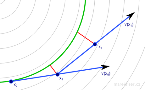
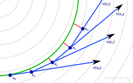
The simplest integrator uses Euler method for integration. The integration step is computed based on current position and vector field value at that position (Equation 1). Figure 8 shows comparison of integration with step dt = 0.5 and dt = 0.25. You can see that shorter time-step results in better results (less error - marked as red lines).

Implementation is literally two lines of code (Code listing 8) and that's the primary reason why I implemented it. However, the down side is that local error (error per step) is proportional to the square of the step size, and the global error (error at a given time) is proportional to the step size.

1
2
3
4

__device__ double4 eulerIntegrate(double3 pos, double dt) {
	float4 v = tex3D(vectorFieldTex, (float)pos.x, (float)pos.y, (float)pos.z);
	return make_double4(dt * v.x, dt * v.y, dt * v.z, v.w);
}

Runge–Kutta 4 integrator

First, I thought that Euler integrator would be enough since CUDA is fast and I can set step size very small. Later in the project it turned out that step size is important for performance and also that lowering step size do not reduce error too much.

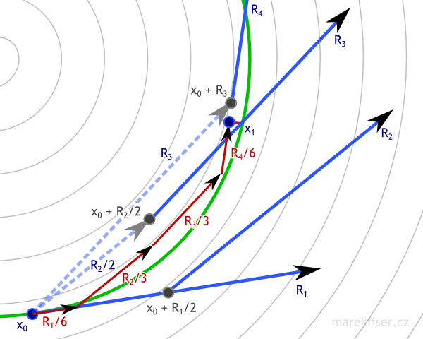
I decided to implement better integrator called Runge–Kutta 4 (Code listing 9). In short, the integrator queries vector field in four cleverly chosen positions and combines results to one step. Equation 6 shows exact equations of integration step and Figure 9 shows the situation visually (please note that this figure was done by hand and actual result could be slightly different). The error of RK4 integrator is smaller by order of magnitude compared to Euler and for some special cases (like circular vector field) might have even no error. For more details how this integrator works please see article on Wikipedia about Runge–Kutta methods.

Figure 9: One step or RK4 integration with dt = 1. Vector field is shown as thin gray lines, green curve represents ground truth, blue arrows are vectors used in computation of RK4 integration, dark red arrows are actual RK4 steps, and small bright red line represents error. Note that RK4 has much smaller error than Euler (Figure 8) even for much bigger time step.

The big advantage of Runge–Kutta integrator is much lower error of integration but it requires more computation power. You can see that in Euler's method for dt=0.5 (Figure 8) has larger error that RK4 method for 4-times larger time step dt = 1 (Figure 9). section Comparison of Euler and RK4 integrators compares both integrators and shows the performance comparison (RK4 is about 4x slower than Euler).

In all following sections is used Runge–Kutta 4 integrator.

1
2
3
4
5
6
7
8
9
10
11
12
13
14
15
16
17
18

__device__ double4 rk4Integrate(double3 pos, double dt) {
	double dtHalf = dt * 0.5;

	float4 k1 = tex3D(vectorFieldTex, (float)pos.x, (float)pos.y, (float)pos.z);
	float4 k2 = tex3D(vectorFieldTex, (float)(pos.x + dtHalf * k1.x),
		(float)(pos.y + dtHalf * k1.y), (float)(pos.z + dtHalf * k1.z));
	float4 k3 = tex3D(vectorFieldTex, (float)(pos.x + dtHalf * k2.x),
		(float)(pos.y + dtHalf * k2.y), (float)(pos.z + dtHalf * k2.z));
	float4 k4 = tex3D(vectorFieldTex, (float)(pos.x + dt * k3.x),
		(float)(pos.y + dt * k3.y), (float)(pos.z + dt * k3.z));

	double dtSixth = dt / 6.0;
	return make_double4(
		dtSixth * (k1.x + 2.0 * ((double)k2.x + k3.x) + k4.x),
		dtSixth * (k1.y + 2.0 * ((double)k2.y + k3.y) + k4.y),
		dtSixth * (k1.z + 2.0 * ((double)k2.z + k3.z) + k4.z),
		(k1.w + 2.0 * ((double)k2.w + k3.w) + k4.w) / 6.0);
}