Realtime visualization of 3D vector fields using CUDA
Chapter 4: Visualization using stream lines and stream tubes
This section shows results of stream line visualization of delta-wing vector field data set. This type of visualization will provide much better understanding of the data than glyphs described in Chapter 2: Visualization using glyphs.
Stream lines
As mentioned in Chapter 3: Vector field integrators for stream line visualization, stream line is trajectory of mass-less particle in vector field. Once we have an integrator, visualization is straight forward. Seed the stream line somewhere in the vector field, compute points at discrete time steps and connect them to a line. Color of the line segment represents the vector magnitude - in our case speed of the air.
The only problem is where to seed the line, there is many possible approaches to this. I decided to seed stream lines on the straight line. User can interactively move this seed-line to explore the vector field.
The first image in Figure 10 shows all features of delta wing dataset. There are primary and secondary vortices rolling above the edges of the wind as well as turbulences behind the wing edge.
Code listing 10 shows simplified kernel for evaluation of array of stream lines. Every stream line is evaluated on separated thread so the true benefit comes with evaluation of more than one line.
Notice that kernel integrates the stream line in double precision but saving the result on single precision.
Also, to save GPU memory there is parameter called geometrySampling which specifies how many
integration samples per emitted geometry sample.
If geometrySampling is set to 1, every step is emitted but for number 2 only every second
point is emitted.
This allows having very short integration step for great precision being be able to save results in limited GPU memory.
1
2
3
4
5
6
7
8
9
10
11
12
13
14
15
16
17
18
19
20
21
22
23
24
25
26
27
28
29
30
31
32
33
34
35
36
37
38
39
40
41
42
43
44
45
46
47
48
49
50
51
__global__ void computeStreamlinesLineKernel(float3* seeds,
			uint seedsCount, double dt, uint maxSteps,
			cudaExtent volumeSize, uint geometrySampling, float3* outVertices,
			uint* outComputedSteps, float3* outVertexColors) {

		uint id = __umul24(blockIdx.x, blockDim.x) + threadIdx.x;
		if (id >= seedsCount) {
			return;
		}

		uint outIndex = id * (maxSteps / geometrySampling + 1);
		// Integration is double precision.
		double3 position = make_double3(seeds[id].x, seeds[id].y, seeds[id].z);

		outVertices[outIndex].x = (float)position.x;
		outVertices[outIndex].y = (float)position.y;
		outVertices[outIndex].z = (float)position.z;
		++outIndex;

		uint geometryStep = geometrySampling;
		uint step = 1;
		for (; step < maxSteps; ++step) {
			if (position.x < 0 || position.y < 0 || position.z < 0
					|| position.x > volumeSize.width
					|| position.y > volumeSize.height
					|| position.z > volumeSize.depth) {
				break;
			}

			double4 dv = rk4Integrate(position, dt);
			position.x += dv.x;
			position.y += dv.y;
			position.z += dv.z;

			--geometryStep;
			if (geometryStep == 0) {
				geometryStep = geometrySampling;

				outVertices[outIndex].x = (float)position.x;
				outVertices[outIndex].y = (float)position.y;
				outVertices[outIndex].z = (float)position.z;
				setColorTo(outVertexColors[outIndex - 1], (float)dv.w);
				++outIndex;
			}
		}

		// Color of the last line point.
		outVertexColors[outIndex - 1] - outVertexColors[outIndex - 2];
		// Save the number of computed line segments.
		outComputedSteps[id] = step / geometrySampling;
	}
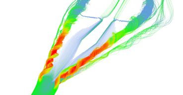
Stream lines seeded at very small area near the tip of the wing. Primary and secondary vortices are nicely visible as well as air moving sideways behind the edge of the wing. 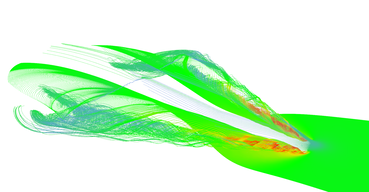
Slightly different setup as previous image. 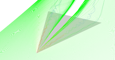
Stream lines seeded at long line in front of the wing. 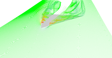
Slightly different setup as previous image.
Stream tubes
Stream lines visualization suffers with very similar problems with ambiguity as line glyphs. It is hard to see the actual position of the line in space in the still image. The fact that there is many lines seeded in straight line helps to imagine orientation but sometimes it is still hard. In the application, you can freely rotate the scene and discover the orientation but results of visualization are usually published as still images.
The trick is to inflate thin lines with some volume and create tubes, stream-tubes. Tubes can be shaded and if there are enough of them close to each other they form nicely shaded surface. Figure 11 shows many images of this type of visualization.
CUDA kernel for computation of stream tubes is very similar to stream lines. The only difference is that we no longer save the position itself but we "extrude" a tube around it. Tube extrusion is done in the plane given by vector from vector field. Tube is constructed only with 5 sides to save as much GPU memory as possible. This sound like very few but combined with smooth shading it is enough. This will ensure that tube will nicely follow stream line in any direction. Code for generation of tubes geometry is shows in Code listing 11.
1
2
3
4
5
6
7
8
9
10
11
12
13
14
15
16
17
18
19
20
21
22
23
24
25
26
27
28
29
30
31
32
33
34
35
36
37
38
39
40
41
42
43
44
45
46
47
48
49
50
51
__device__ void createTubeBaseVertices(float3 pos, float3 v,
		float radius, uint baseIndex, float3 color,
		float3* outVetrices, float3* outNormals, float3* outColors) {

	float3 xAxis = normalize(findPerpendicular(v));
	float3 yAxis = normalize(cross(v, xAxis));

	// x * cos(0) + y * sin(0)
	outNormals[baseIndex] = xAxis;
	outVetrices[baseIndex] = pos + xAxis * radius;
	outColors[baseIndex] = color;
	++baseIndex;

	// x * cos(72) + y * sin(72)
	v = 0.3090f * xAxis + 0.9511f * yAxis;
	outNormals[baseIndex] = v;
	outVetrices[baseIndex] = pos + v * radius;
	outColors[baseIndex] = color;
	++baseIndex;

	// x * cos(144) + y * sin(144)
	v = -0.8090f * xAxis + 0.5878f * yAxis;
	outNormals[baseIndex] = v;
	outVetrices[baseIndex] = pos + v * radius;
	outColors[baseIndex] = color;
	++baseIndex;

	// x * cos(216) + y * sin(216)
	v = -0.8090f * xAxis - 0.5878f * yAxis;
	outNormals[baseIndex] = v;
	outVetrices[baseIndex] = pos + v * radius;
	outColors[baseIndex] = color;
	++baseIndex;

	// x * cos(288) + y * sin(288)
	v = 0.3090f * xAxis - 0.9511f * yAxis;
	outNormals[baseIndex] = v;
	outVetrices[baseIndex] = pos + v * radius;
	outColors[baseIndex] = color;
}

__device__ void createTubeIndices(uint vertexBaseId, uint baseFaceId, uint3* outFaces) {

	for (uint i = 0; i < 5; ++i) {
		uint iNext = (i + 1) % 5;
		outFaces[baseFaceId++] = make_uint3(vertexBaseId + i,
			vertexBaseId + iNext, vertexBaseId - 5 + iNext);
		outFaces[baseFaceId++] = make_uint3(vertexBaseId + i,
			vertexBaseId - 5 + i, vertexBaseId - 5 + iNext);
	}
}
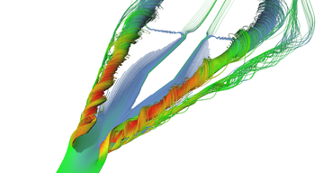
Stream tubes showing the main features of the delta-wing dataset - primary and secondary vortices and air going sideways behind the back edge of the wing. 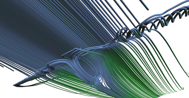
Detail on the back of the wing from the bottom. You can clearly see the vortex behind the box on the wing (the wing and the box is not shown). 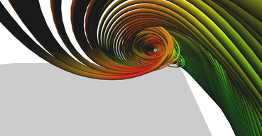
Detail of the primary vortex. 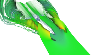
Another visualization of the datasets using stream-tubes. 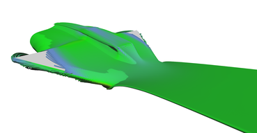
Air hitting the bottom of the wing revealing the aerodynamic box. Notice how air rolls over the edges of the box. 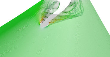
Another visualization of the datasets using stream-tubes. 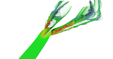
Narrow stream of air hitting the tip of the wing. 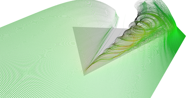
Row of stream-tubes seeded among the wing edge. 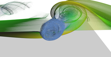
Recirculation bubble visualization. 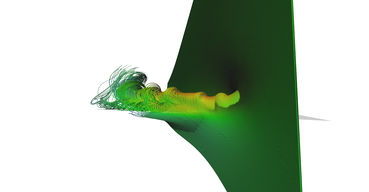
Vertical seeding of stream-tubes.
Adaptive stream lines
The next step towards high quality visualization is seeding the stream lines adaptively. The problem of regular seeding is that by increasing the number of lines some non-interesting areas (i.e. where flow is laminar) have too many lines but interesting areas (i.e. where flow is turbulent) could benefit from more lines.
Figure 12 shows a comparison between regular and adaptive stream lines seeding. It is nicely visible that areas with linear flow are subdivided significantly less than areas with vortices.

Regular vs. adaptive (pair 1, regular). 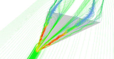
Regular vs. adaptive (pair 1, adaptive). Area near the tip of the wing is sampled much more because air is forming vortices there. 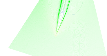
Regular vs. adaptive (pair 2, regular). 
Regular vs. adaptive (pair 2, adaptive). Adaptive seeding revealed important features. 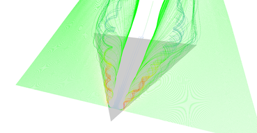
Regular vs. adaptive (pair 3, regular). 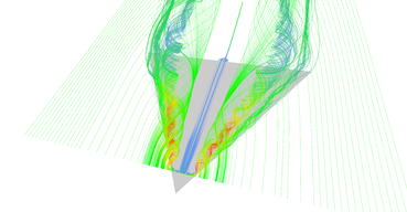
Regular vs. adaptive (pair 3, adaptive). 
Regular vs. adaptive (pair 4, regular). 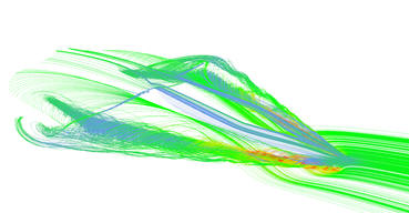
Regular vs. adaptive (pair 4, adaptive). 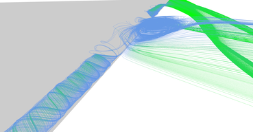
Regular vs. adaptive (pair 5, regular). 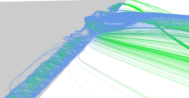
Regular vs. adaptive (pair 5, adaptive).
True challenge is implement adaptive algorithm on GPU. It is very hard performance costly to do thread communication on GPU. My algorithm uses two different CUDA kernels, one for control of adaptivity and second for evaluation of stream lines themselves. Both algorithms are alternately invoked by CPU. This makes effectivity of overall algorithm worse that non-adaptive version but results are much better and overall slow-down is not very significant.
Also, memory management is not simple because you need to allocate all memory needed for GPU run before you start the kernel. Algorithm is designed in a way that space for maximum amount of lines is allocated and then adaptive algorithm is filling it till it reaches the limit.
The adaptivity is implemented as subdivision. Starting with two stream lines, algorithm is adding new seeds in between stream lines which diverged (i.e. are too far from each other). Code listing 12 shows kernel for coordination of adaptivity. Input is array of line pair indices which are neighbors and needs to be considered for divergence. Divergence is determined by 32 samples among stream lines. If any of those samples is further than maximum allowed distance, new seed is seeded in between them. Output is list of neighboring line pairs as well. Notice that clever usage of line pair indices allows subdividing lines which are at arbitrary positions in memory buffer.
This process tends to be quite slow at the beginning because number of new lines in n-th iteration is 2n. To speed up start, number of added seeds is determined based on maximal distance between two stream lines.
1
uint newLines = (uint)sqrtf(maxDist / maxAllowedLineDist);
Another nice feature of this code is usage of atomic operations for use of static array as dynamic array. Because it is impossible to know in advance how many seeds new will be produced by subdivision kernel, array is allocated for maximum number of seeds and every thread tries to add one more. The variable responsible for tracking the number of elements in the array is atomically incremented and if the count is smaller than maximum allowed number of elements, new seed is added. Otherwise, variable is atomically decremented.
Figure 13 shows progression of adaptive stream line seeding algorithm iteration by iteration. Lines are very thin and hard to see, please click the thumbnails for larger image.
1
2
3
4
5
6
7
8
9
10
11
12
13
14
15
16
17
18
19
20
21
22
23
24
25
26
27
28
29
30
31
32
33
34
35
36
37
38
39
40
41
42
43
44
45
46
47
48
49
50
51
52
53
54
55
56
__global__ void computeLineAdaptiveExtensionKernel(
		float maxAllowedLineDist, uint2* linePairs, uint linePairsCount,
		float3* lineVertices, uint verticesPerLine, uint verticesPerSample,
		uint* lineLengths, float3* seeds, uint2* outLinePairs,
		uint* outPairsIndex, uint* outLinesIndex, uint linesMaxCount) {

	uint id = __umul24(blockIdx.x, blockDim.x) + threadIdx.x;
	if (id >= linePairsCount) {
		return;
	}

	uint2 currPair = linePairs[id];
	uint outPairIndex = atomicAdd(outPairsIndex, 1);
	// Preserve original pair.
	outLinePairs[outPairIndex].x = currPair.x;
	outLinePairs[outPairIndex].y = currPair.y;

	uint count = min(lineLengths[currPair.x], lineLengths[currPair.y]);
	if (count < 2) {
		return;  // One of lines too short.
	}

	// Test 32 samples for divergence.
	float maxDist = 0;
	for (uint i = 0; i < count; i += count / 32) {
		float3 v1 = lineVertices[currPair.x * verticesPerLine + i * verticesPerSample];
		float3 v2 = lineVertices[currPair.y * verticesPerLine + i * verticesPerSample];
		maxDist = max(maxDist, length(v1 - v2));
	}

	if (maxDist < maxAllowedLineDist) {
		return;  // Lines do not diverged.
	}

	uint newLines = (uint)sqrtf(maxDist / maxAllowedLineDist);

	uint outLineIndex = atomicAdd(outLinesIndex, newLines);
	if ((outLineIndex + newLines) >= linesMaxCount) {
		atomicAdd(outLinesIndex, -newLines);
		return;  // Not enough space for new seeds.
	}

	float3 seedStep = (seeds[currPair.y] - seeds[currPair.x]) / (newLines + 1);

	uint lastOutPairIndex = outPairIndex;
	for (uint i = 0; i < newLines; ++i) {
		seeds[outLineIndex + i] = seeds[currPair.x] + (i + 1) * seedStep;
		// Insert new pair (like in linked-list).
		uint outPairIndex = atomicAdd(outPairsIndex, 1);
		outLinePairs[lastOutPairIndex].y = outLineIndex + i;
		outLinePairs[outPairIndex].x = outLineIndex + i;
		outLinePairs[outPairIndex].y = currPair.y;

		lastOutPairIndex = outPairIndex;
	}
}
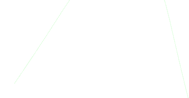
Step 1 of adaptive seeding algorithm. 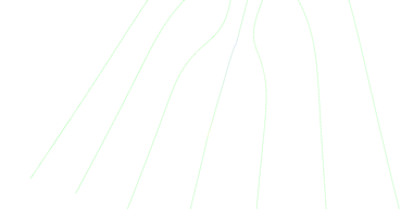
Step 2 of adaptive seeding algorithm. 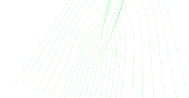
Step 3 of adaptive seeding algorithm. 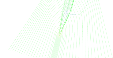
Step 4 of adaptive seeding algorithm. 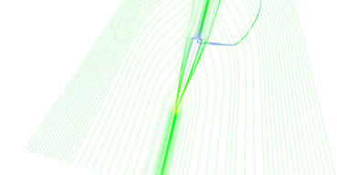
Step 5 of adaptive seeding algorithm. 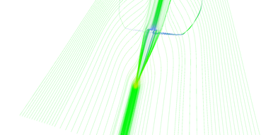
Step 6 of adaptive seeding algorithm. 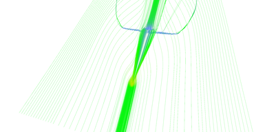
Step 7 of adaptive seeding algorithm. 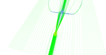
Step 8 of adaptive seeding algorithm.